Thermoelasticity

This tutorial develops a complete quasi-static thermoelastic analysis of PBE0 dolomite. It begins with a quasi-harmonic pressure-temperature result and a series of static elastic tensors, calibrates a reusable cold finite-strain model, and then evaluates that model at a single state, on a rectangular pressure-temperature grid, and along a continental depth profile.

The tutorial deliberately follows the staged design of Quantas:

QHA input or result
        +
static Cij(V) series
        |
        v
model calibration
        |
        +--> one P-T state --> Elasticity/SEISMIC input
        |
        +--> rectangular P-T grid --> HDF5 + CSV + contour plots
        |
        +--> geological profile --> HDF5 + CSV + depth plots

The scientific theory is described in Thermoelasticity. The operational model and validation policies are described in Thermoelasticity: implementation and workflow.

Scientific objective

The goal is to determine the evolution of the dolomite elastic tensor under combined pressure and temperature using the quasi-static approximation,

\[C^T_{IJ}(P,T) \simeq C^{\mathrm c}_{IJ}\!\left[V_{\mathrm{QHA}}(P,T)\right].\]

The cold elastic model is calibrated from static second-order elastic coefficients sampled at several volumes. The QHA calculation supplies the equilibrium volume and thermodynamic quantities at finite pressure and temperature. Quantas can then reconstruct:

• the isothermal tensor \(C^T(P,T)\);

• the adiabatic tensor \(C^S(P,T)\), when the required QHA fields exist;

• density and equilibrium volume;

• propagated fit and volume uncertainties;

• mechanical-stability diagnostics;

• extrapolation masks for the QHA coordinate domain and elastic-volume domain.

This workflow does not calculate the explicit strain derivatives of the phonon frequencies. Temperature enters the cold tensor through the QHA volume, followed by the explicit isothermal-to-adiabatic conversion where available.

Dataset

The tutorial combines two curated datasets.

Static elastic series

The thermoelastic input contains eleven CRYSTAL calculations from -6 to 20 GPa. Each calculation includes:

• the static electronic energy;

• primitive-cell volume and density;

• a complete pressure-corrected Wallace stiffness tensor;

• the lattice and ordered atomic structure;

• tensor-frame normalization metadata.

The normalized input is distributed here:

Download the dolomite thermoelastic YAML

The original CRYSTAL outputs are retained under examples/thermoelasticity/crystal_outputs. The list file contains:

dol_pbe0_soec_p-06.out
dol_pbe0_soec_p-04.out
dol_pbe0_soec_p-02.out
dol_pbe0_soec_p+00.out
dol_pbe0_soec_p+02.out
dol_pbe0_soec_p+04.out
dol_pbe0_soec_p+06.out
dol_pbe0_soec_p+08.out
dol_pbe0_soec_p+10.out
dol_pbe0_soec_p+15.out
dol_pbe0_soec_p+20.out

The CRYSTAL PRESSURE keyword is essential. It ensures that the reported coefficients already contain the hydrostatic pre-stress correction required for wave propagation and thermoelastic reconstruction. Quantas must not apply the same correction a second time.

QHA dataset

The QHA input contains seven volumes, 27 q-points, and 30 phonon modes for the primitive dolomite cell:

Download the dolomite QHA YAML

The tutorial evaluates the QHA model from 300 to 1800 K and from 0 to 10 GPa. This wider temperature interval is needed because the geological profile later reaches approximately 1380 K.

Before continuing

A reliable thermoelastic calculation needs more than two files with compatible names. Check the following scientific conditions first.

1. The QHA and elastic calculations describe the same normalized cell.

2. Static elastic tensors are sampled over a volume interval broad enough to contain the QHA equilibrium volumes of interest.

3. Every elastic tensor uses one common Cartesian frame.

4. The same Voigt and shear-strain convention is used throughout.

5. The static tensors include the appropriate pressure correction.

6. The QHA result contains \(C_V\) and the thermal-expansion tensor if an adiabatic tensor is required.

7. The requested pressure-temperature states are meaningful for the material; Quantas does not determine phase stability or decomposition boundaries.

Stage 1: generating the thermoelastic input

Starting from the CRYSTAL outputs, create the normalized YAML with:

cd examples/thermoelasticity/crystal_outputs

quantas thermoelasticity inpgen dol_pbe0_soec.txt \
    --list \
    --jobname "Dolomite PBE0 QSA thermoelasticity" \
    --output ../dol_pbe0_thermoelastic.yaml \
    --force

During input generation Quantas:

• reads every elastic tensor and its pressure;

• sorts the points consistently;

• checks ordered-atom correspondence;

• determines the elastic symmetry;

• co-rotates sampled tensors to a single reference frame;

• stores the original and normalized frame metadata.

The beginning of the resulting file records the scientific conventions:

schema:
  name: quantas-thermoelastic-input
  version: '1.0'
job: Dolomite PBE0 QSA thermoelasticity
method: quasistatic
interface: crystal
conventions:
  strain: eulerian-finite-strain
  stiffness: wallace-hydrostatic-stress-strain
  prestress: applied-by-crystal-pressure-keyword
  tensor_orientation: crystal

The YAML is intentionally readable. It is also the normalized contract used by both CLI and Python frontends.

Stage 2: preparing the QHA result

The QHA workflow is described in detail in Quasi-Harmonic Approximation. For this tutorial, run:

quantas qha run examples/qha/crystal-phonons/dol_pbe0.yaml \
    --scheme freq \
    --minimization poly \
    --thermal-expansion mixed_derivative \
    --temperature 300 1800 100 \
    --pressure 0 10 2 \
    --energy-degree 3 \
    --frequency-degree 3 \
    --output dolomite_qha.hdf5 \
    --report dolomite_qha.log \
    --verbosity standard \
    --no-progress \
    --force

The resulting archive supplies the equilibrium-volume field \(V(P,T)\), density normalization, \(C_V\), and the Cartesian thermal-expansion tensor needed by the later reconstruction.

The QHA calculation reports 16 temperatures and 6 pressures. Selected zero-pressure values are:

T (K)	V (ų)	\(K_T\) (GPa)	\(\alpha_V\) (10⁻⁵ K⁻¹)
300	109.1678	90.218	2.2953
800	110.7406	80.819	3.2812
1200	112.3460	70.932	3.9607

The cell expands and softens as temperature rises. Pressure reverses part of this expansion and increases the bulk modulus.

Stage 3: calibrating the cold finite-strain model

Calibration is performed once. The resulting fit archive can then be reused for many points, grids, and profiles.

quantas thermoelasticity run \
    examples/thermoelasticity/dol_pbe0_thermoelastic.yaml \
    dolomite_qha.hdf5 \
    --reference-eos BM3 \
    --finite-strain-order 3 \
    --adiabatic auto \
    --validation standard \
    --plot \
    --plot-output dolomite_fit_plots \
    --plot-preset publication \
    --output dolomite_fit.hdf5 \
    --report dolomite_fit.log \
    --verbosity standard \
    --no-progress \
    --force

Scientific choices

--reference-eos BM3

Fit the static energy-volume data with a third-order Birch–Murnaghan EOS. The fitted \(V_0\), \(K_0\), and \(K'_0\) are shared by all component fits.

--finite-strain-order 3

Retain the quadratic finite-strain term in the cold elastic expansion.

--adiabatic auto

Preserve the isothermal QSA model and prepare the archived thermodynamic fields needed to construct \(C^S\) during point, grid, or profile analysis.

--validation standard

Keep supported fits, report cautionary conditions, and reject only scientifically unacceptable failures.

Reference EOS

The report gives:

Static reference EOS
EOS               BM3
V0                107.8981 +/- 0.0426 A^3
K0                 93.2830 +/- 0.7105 GPa
Kprime              3.7556 +/- 0.2667
Fit quality          good
R squared            1.0000

The reference EOS is fitted from the static electronic energies. It is not the finite-temperature QHA EOS.

Independent components

Dolomite has trigonal-low elastic symmetry in the selected Cartesian frame. The active independent components are:

C11  C12  C13  C14  C15  C33  C44

All seven component fits are classified as supported for this dataset. A supported classification means that the volume span, design conditioning, leave-one-out behavior, and residual diagnostics satisfy the selected quality policy. It does not mean that the model is exact or universally extrapolatable.

A small warning is emitted because the mass inferred independently from the CRYSTAL density-volume pairs varies by 0.001712%. The spread is small enough for the normalized-cell mass to remain usable, but the provenance is retained rather than silently discarded.

Understanding the fit figure

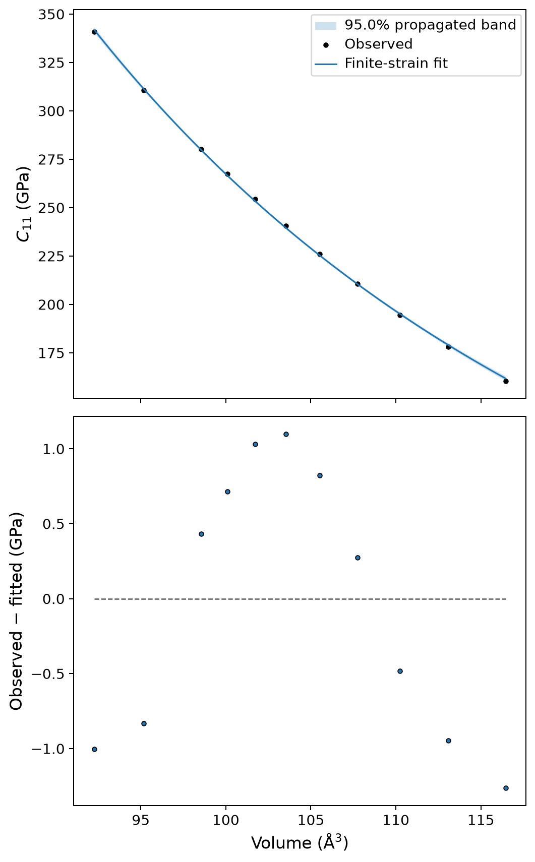
Observed and fitted \(C_{11}(V)\) with residuals and the propagated 95% confidence band.

The stiffness decreases as the volume expands. The residuals remain close to zero compared with the full \(C_{11}\) range, but they are not random noise with known experimental variance: the source calculations provide no SOEC uncertainties, so the report labels the residual sum of squares as unweighted. The confidence band therefore describes propagated parameter uncertainty under the fitted model, not a complete uncertainty budget for the electronic- structure calculation.

Why the fit archive contains no reconstructed tensor grid

Immediately after calibration, the report states:

Grid reconstruction                 deferred
Grid tensors                        0
Isothermal tensor condition         absent
Adiabatic tensor condition          absent

This is intentional. run calibrates a reusable scientific model; it does not assume which P–T states the user wants to analyze. Reconstruction occurs in the later analysis stage.

Inspecting the calibrated archive

quantas thermoelasticity inspect dolomite_fit.hdf5

The relevant summary is:

Stage                 model calibration
Reference EOS         BM3
Independent Cij       C11 C12 C13 C14 C15 C33 C44
Tensor conditions     isothermal, adiabatic on analysis
Frame status          normalized
P support (GPa)       0-10
T support (K)         300-1800
Fit quality           supported=7

The pressure and temperature support shown here comes from the archived QHA coordinates. Elastic-volume support is checked independently at every reconstructed state.

Stage 4: evaluating one state

Evaluate the adiabatic tensor at 5 GPa and 800 K:

quantas thermoelasticity analysis point dolomite_fit.hdf5 5 800 \
    --tensor-condition adiabatic \
    --extrapolation fail \
    --output dolomite_5GPa_800K.dat \
    --force

The point table is:

Thermoelastic point (adiabatic)
Pressure              5.0000 GPa
Temperature           800.00 K
Volume                104.9943 A^3
Density               2908.74 kg m^-3
C11_S                 230.2963 +/- 0.3460 GPa
C12_S                  82.1914 +/- 0.4334 GPa
C13_S                  70.2862 +/- 0.2907 GPa
C14_S                  20.4173 +/- 0.3598 GPa
C15_S                 -14.6793 +/- 0.1088 GPa
C33_S                 126.7214 +/- 0.4290 GPa
C44_S                  45.4699 +/- 0.2486 GPa
Mechanically stable   True
QHA extrapolated      False
Elastic extrapolated  False

The two extrapolation flags are independent:

QHA extrapolated

The requested pressure or temperature lies outside the archived QHA coordinate range.

Elastic extrapolated

The reconstructed QHA volume lies outside the sampled static elastic-volume interval.

Both are false here, and the full Wallace stiffness matrix is positive definite.

Reusable Elasticity/SEISMIC input

The output file contains the complete symmetric \(6\times6\) adiabatic tensor followed by the QHA-consistent density:

Dolomite PBE0 QSA thermoelasticity | P=5 GPa, T=800 K, C^S
    230.296285   82.191419   70.286248   20.417263  -14.679291    0.000000
     82.191419  230.296285   70.286248  -20.417263   14.679291    0.000000
     70.286248   70.286248  126.721432   -0.000000    0.000000    0.000000
     20.417263  -20.417263   -0.000000   45.469942   -0.000000   14.679291
    -14.679291   14.679291    0.000000   -0.000000   45.469942   20.417263
      0.000000    0.000000    0.000000   14.679291   20.417263   74.052433
2908.73674895

Download the generated state input

It can be passed directly to the other tensor workflows:

quantas elasticity run dolomite_5GPa_800K.dat
quantas seismic run dolomite_5GPa_800K.dat

This is the simplest practical example of Quantas interoperability.

Stage 5: evaluating a pressure-temperature grid

Construct a grid from 0 to 10 GPa and 300 to 1200 K:

quantas thermoelasticity analysis grid dolomite_fit.hdf5 \
    --pressure 0 10 2 \
    --temperature 300 1200 100 \
    --tensor-condition both \
    --extrapolation fail \
    --output dolomite_grid.hdf5 \
    --table-output dolomite_grid.csv \
    --table-format csv \
    --uncertainties \
    --force

The HDF5 archive stores full \(6\times6\) tensors. The wide CSV retains only symmetry-independent components, avoiding redundant columns. The first rows contain fields such as:

pressure_GPa,temperature_K,volume_A3,density_kg_m3,
C11_T_GPa,sigma_C11_T_GPa,...,C11_S_GPa,sigma_C11_S_GPa,...,
qha_extrapolated,elastic_extrapolated,adiabatic_valid,
mechanically_stable,minimum_stiffness_eigenvalue_GPa

At 300 K:

P (GPa)	V (ų)	\(C^T_{11}\) (GPa)	\(C^T_{33}\) (GPa)	\(C^T_{44}\) (GPa)
0	109.1678	201.5613	110.5776	40.1602
4	104.8363	230.1133	125.9168	45.6836
8	101.2062	257.4719	140.2764	50.8689

Compression stiffens every listed component. Temperature produces the opposite trend at fixed pressure because thermal expansion moves the system to a larger equilibrium volume.

Download the complete grid table

Pressure-temperature maps

Generate two isothermal stiffness maps:

quantas thermoelasticity plot pt dolomite_grid.hdf5 \
    --component C11 \
    --component C33 \
    --tensor-condition isothermal \
    --quantity value \
    --layout facets \
    --levels 12 \
    --isolines \
    --isoline-labels \
    --preset publication \
    --output dolomite_pt_plots \
    --format png \
    --dpi 180

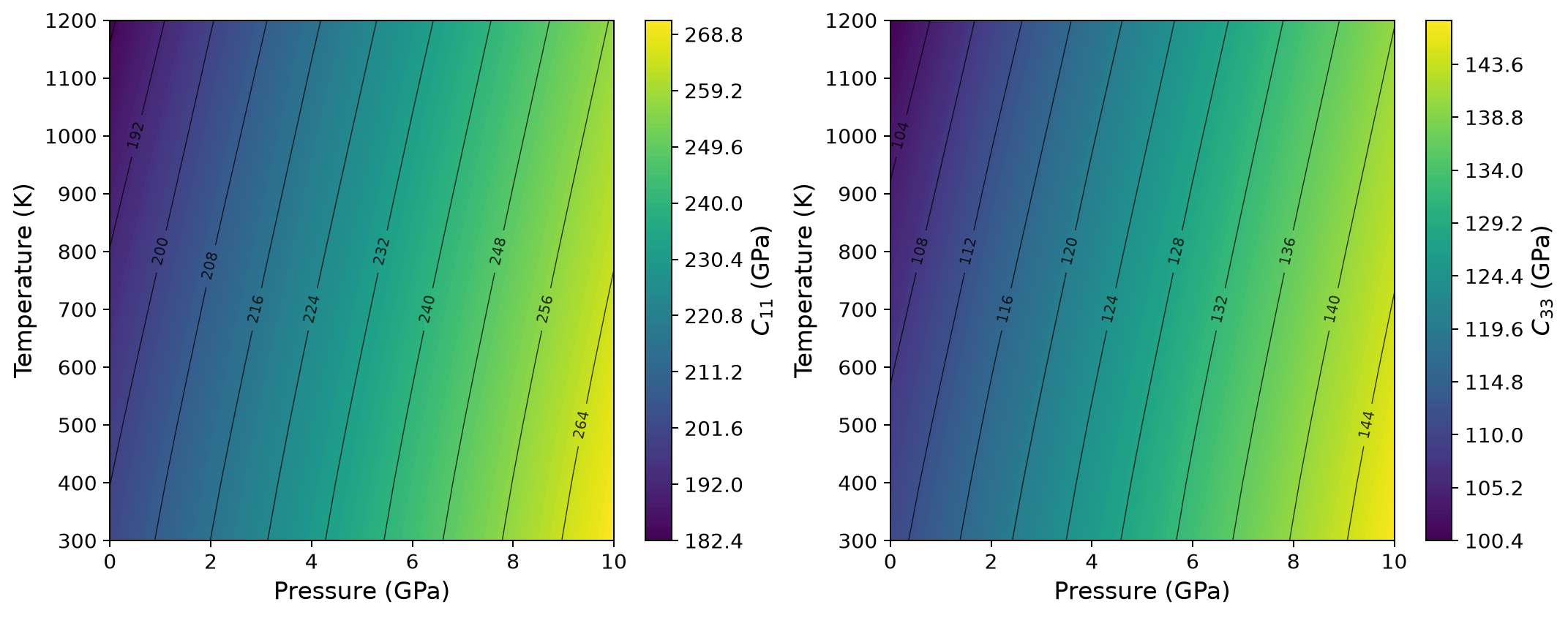
Isothermal \(C_{11}\) and \(C_{33}\) over the analyzed P–T grid.

The nearly vertical contour orientation shows that pressure is the dominant control over this domain. Their finite tilt records thermal softening. The relative slopes differ between \(C_{11}\) and \(C_{33}\), so a scalar bulk-modulus trend cannot replace the tensorial analysis.

Stage 6: comparing isothermal and adiabatic tensors

At constant pressure, compare \(C^T\) and \(C^S\):

quantas thermoelasticity plot compare dolomite_grid.hdf5 \
    --component C11 \
    --component C33 \
    --pressure 0 \
    --layout facets \
    --preset publication \
    --output dolomite_compare_plots \
    --format png \
    --dpi 180

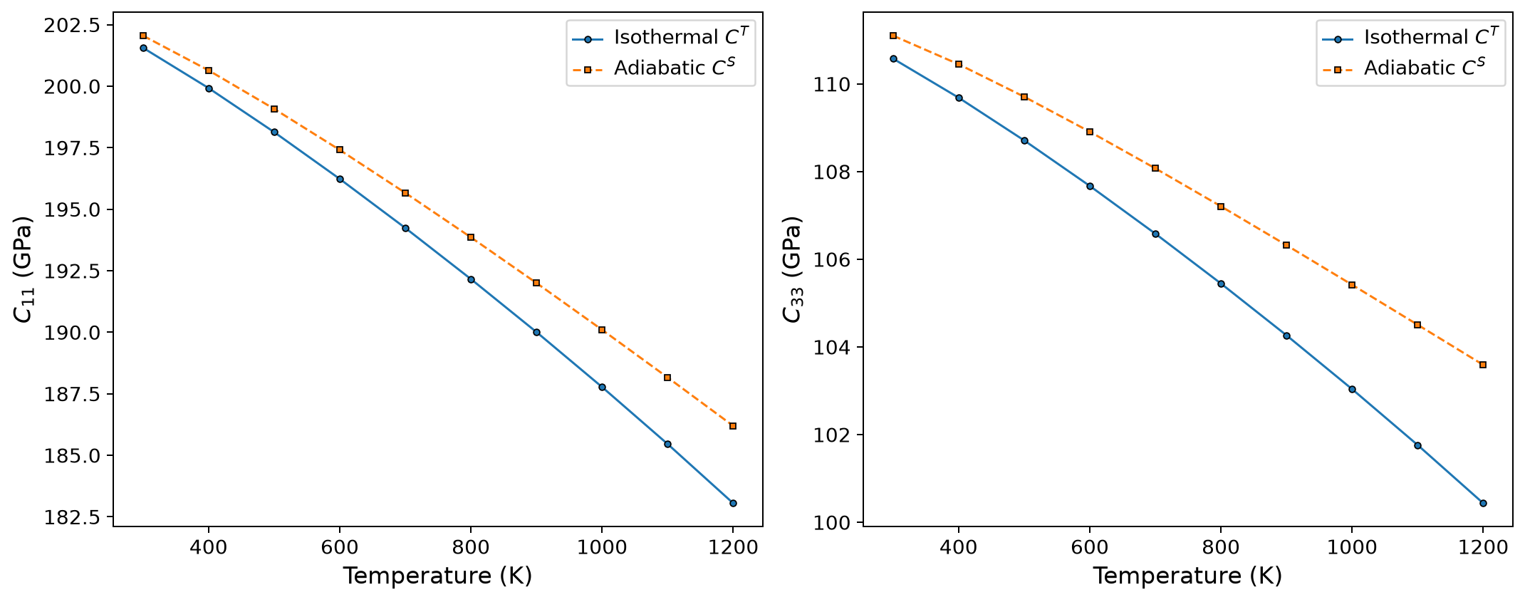
Isothermal and adiabatic \(C_{11}\) and \(C_{33}\) at 0 GPa.

Selected values are:

T (K)	\(C^T_{11}\)	\(C^S_{11}\)	\(C^T_{33}\)	\(C^S_{33}\)
300	201.5613	202.0548	110.5776	111.1018
800	192.1630	193.8586	105.4477	107.2084
1200	183.0517	186.1955	100.4355	103.5912

All values are in GPa. The adiabatic tensor is stiffer for the normal components shown, and the separation increases with temperature. In this example \(C_{44}\) is unchanged by the adiabatic correction because the thermal-stress vector and symmetry constrain the correction to the relevant normal/coupled subspace.

Stage 7: evaluating a geological profile

The profile is deliberately separated from the rectangular grid. It evaluates only the states required by the geological path.

Profile definition

The tutorial uses PREM pressure and a layered steady conductive continental temperature model from 0 to 80 km:

Download the profile specification

The profile is an illustrative demonstration of the accepted formalism. The thermal parameters must be replaced by a documented regional model before quantitative geological interpretation. Quantas also does not test whether dolomite remains the stable phase over the entire path.

The pressure and temperature models are independent:

pressure:
  model: prem

temperature:
  model: continental-conductive
  surface_temperature_K: 300.0
  surface_heat_flow_mW_m2: 55.0
  layers:
    - name: upper crust
      thickness_km: 15.0
      conductivity_W_mK: 2.5
      heat_production_uW_m3: 0.8
    - name: lower crust
      thickness_km: 20.0
      conductivity_W_mK: 2.5
      heat_production_uW_m3: 0.4
    - name: lithospheric mantle
      thickness_km: 45.0
      conductivity_W_mK: 3.3
      heat_production_uW_m3: 0.02

Run the profile analysis:

quantas thermoelasticity analysis profile dolomite_fit.hdf5 \
    --profile-spec \
    examples/thermoelasticity/dolomite_continental_profile.yaml \
    --tensor-condition both \
    --extrapolation fail \
    --output dolomite_profile.hdf5 \
    --table-output dolomite_profile.csv \
    --table-format csv \
    --uncertainties \
    --plot \
    --force

The profile contains 45 depth points because layer boundaries and other critical depths are inserted in addition to the regular 2 km spacing.

Selected profile states

Depth (km)	P (GPa)	T (K)	V (ų)	\(C^S_{11}\)	\(C^S_{33}\)	\(C^S_{44}\)
0	0.000	300	109.1678	202.0548	111.1018	40.1602
15	0.339	594	109.6213	199.9423	110.2774	39.6202
35	0.961	906	109.8861	199.0656	110.1504	39.3080
80	2.458	1377	109.5623	202.0226	112.2875	39.6900

Stiffness values are in GPa. The volume initially increases because thermal expansion dominates the pressure increase. At greater depth the pressure term becomes strong enough to reverse part of that expansion. The tensor response is consequently non-monotonic:

• \(C^S_{11}\) reaches a minimum change of approximately -1.48% near 35 km and almost returns to its surface value at 80 km;

• \(C^S_{33}\) reaches a shallow minimum and ends approximately 1.07% above its surface value;

• \(C^S_{44}\) reaches approximately -2.12% near 35 km and remains about 1.17% below its surface value at 80 km.

This is precisely why a coupled P–T path is more informative than a pressure- only or temperature-only curve.

Download the complete profile table

Relative profile plot

quantas thermoelasticity plot profile dolomite_profile.hdf5 \
    --profile-name dolomite-continental-demo \
    --component C11 \
    --component C33 \
    --component C44 \
    --tensor-condition adiabatic \
    --mode relative \
    --layout overlay \
    --uncertainty none \
    --pressure-axis \
    --color-by component \
    --preset publication \
    --output dolomite_profile_plots \
    --format png \
    --dpi 180

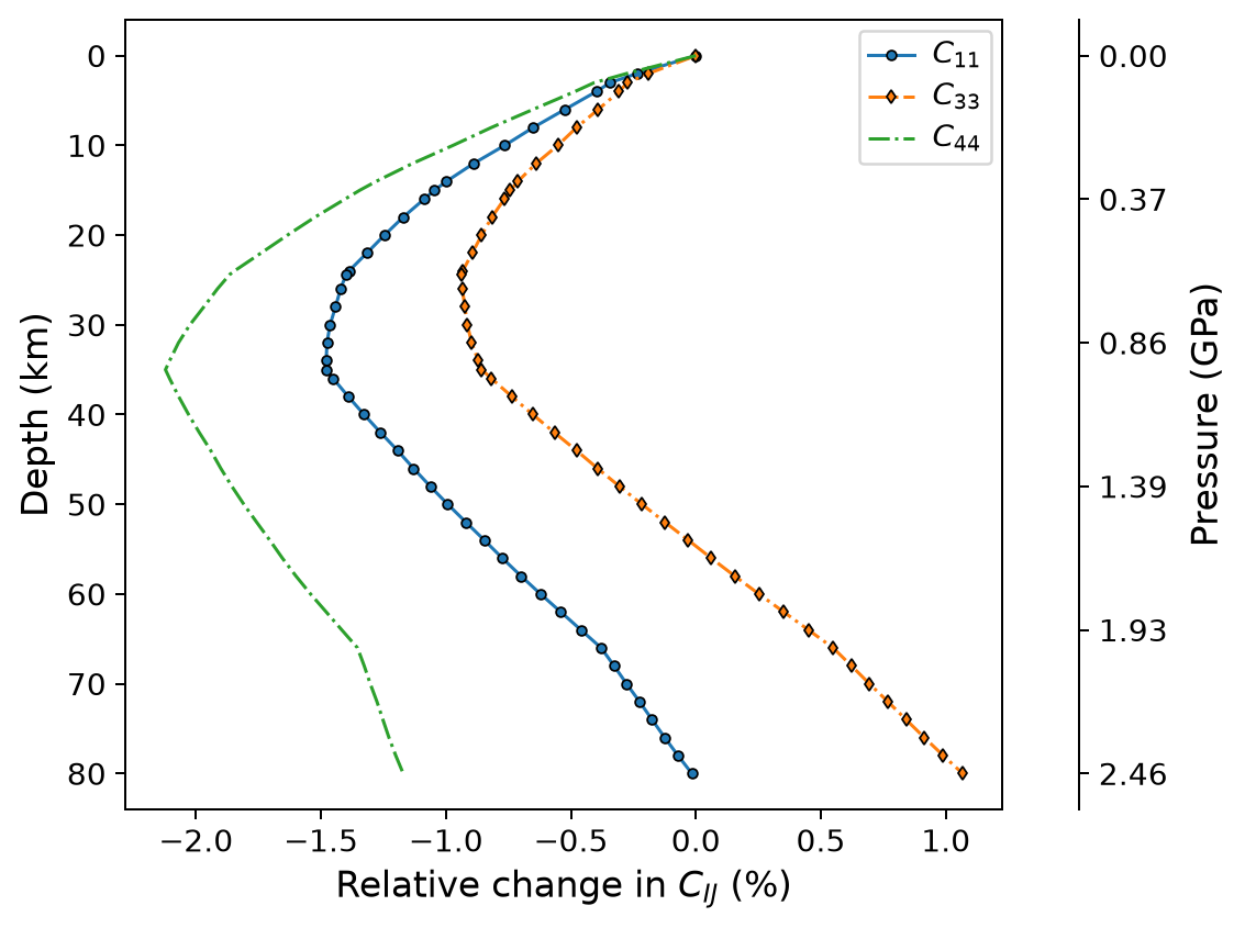
Relative changes in \(C^S_{11}\), \(C^S_{33}\), and \(C^S_{44}\) along the illustrative continental path.

The profile plot emphasizes relative response and therefore omits uncertainty bands for the three-component overlay. Absolute values and uncertainties remain available in the CSV and HDF5 products.

Checking the P–T and volume domain

quantas thermoelasticity plot domain dolomite_profile.hdf5 \
    --profile-name dolomite-continental-demo \
    --profiles \
    --extrapolation \
    --color-profiles-by-depth \
    --preset publication \
    --output dolomite_domain_plots \
    --format png \
    --dpi 180

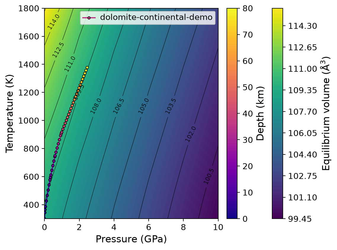
The geological path over the archived QHA equilibrium-volume field.

The path lies inside the QHA coordinate domain and inside the sampled elastic- volume interval, so no extrapolation region is marked. The background shows that the path crosses nearly constant-volume contours: temperature-driven expansion is progressively countered by pressure-driven compression.

Running the same workflow from Python

The complete public-API script is distributed with the examples:

Download the Thermoelasticity API script

"""Run the complete dolomite thermoelasticity tutorial through the public API.

The script expects the normalized thermoelastic input, the dolomite QHA YAML,
and the composed continental profile distributed with Quantas.  It performs
QHA, calibrates the quasi-static elastic model, evaluates a point, a P--T grid,
and a depth profile, writes HDF5/table products, and renders selected figures.

Examples
--------
Run from the project root::

    python examples/thermoelasticity/tutorial_api.py \
        --output-dir thermoelasticity_tutorial
"""

from __future__ import annotations

import argparse
from pathlib import Path

import numpy as np

from quantas.api import qha, rendering, thermoelasticity


def parser() -> argparse.ArgumentParser:
    """Return the command-line parser for the standalone API tutorial."""
    result = argparse.ArgumentParser(description=__doc__)
    result.add_argument(
        "--thermoelastic-input",
        type=Path,
        default=Path("examples/thermoelasticity/dol_pbe0_thermoelastic.yaml"),
    )
    result.add_argument(
        "--qha-input",
        type=Path,
        default=Path("examples/qha/crystal-phonons/dol_pbe0.yaml"),
    )
    result.add_argument(
        "--profile-spec",
        type=Path,
        default=Path(
            "examples/thermoelasticity/dolomite_continental_profile.yaml"
        ),
    )
    result.add_argument(
        "--output-dir",
        type=Path,
        default=Path("thermoelasticity_tutorial"),
    )
    return result


def main() -> None:
    """Execute the complete API workflow and write tutorial products."""
    args = parser().parse_args()
    args.output_dir.mkdir(parents=True, exist_ok=True)
    figures = args.output_dir / "figures"
    figures.mkdir(parents=True, exist_ok=True)

    qha_result = qha.run(
        args.qha_input,
        options=qha.Options(
            temperature_min=300.0,
            temperature_max=1800.0,
            temperature_step=100.0,
            pressure_min=0.0,
            pressure_max=10.0,
            pressure_step=2.0,
            scheme="freq",
            minimization="poly",
            energy_degree=3,
            frequency_degree=3,
            thermal_expansion_method="mixed_derivative",
        ),
    )
    qha_report = rendering.render_tables(qha.build_report(qha_result))
    qha.write_result(
        qha_result,
        args.output_dir / "dolomite_qha.hdf5",
        report_text=qha_report,
    )
    (args.output_dir / "dolomite_qha.log").write_text(
        qha_report,
        encoding="utf-8",
    )

    fit_result = thermoelasticity.run(
        args.thermoelastic_input,
        qha_result,
        options=thermoelasticity.Options(
            reference_eos="BM3",
            finite_strain_order=3,
            adiabatic_mode="auto",
            quality_policy="warn",
            report_level="standard",
        ),
    )
    fit_report = rendering.render_tables(
        thermoelasticity.build_report(fit_result, level="standard")
    )
    thermoelasticity.write_result(
        fit_result,
        args.output_dir / "dolomite_fit.hdf5",
        report_text=fit_report,
    )
    (args.output_dir / "dolomite_fit.log").write_text(
        fit_report,
        encoding="utf-8",
    )

    point_result = thermoelasticity.analyze_grid(
        fit_result,
        pressure=np.asarray([5.0], dtype=np.float64),
        temperature=np.asarray([800.0], dtype=np.float64),
        extrapolation_policy="fail",
    )
    point_payload = thermoelasticity.get_result(point_result)
    print(
        rendering.render_tables(
            [thermoelasticity.point_table(point_payload, tensor_condition="adiabatic")]
        )
    )
    thermoelasticity.write_state_input(
        point_payload,
        args.output_dir / "dolomite_5GPa_800K.dat",
        tensor_condition="adiabatic",
        overwrite=True,
    )

    grid_result = thermoelasticity.analyze_grid(
        fit_result,
        pressure=thermoelasticity.regular_grid(0.0, 10.0, 2.0),
        temperature=thermoelasticity.regular_grid(300.0, 1200.0, 100.0),
        extrapolation_policy="fail",
    )
    grid_payload = thermoelasticity.get_result(grid_result)
    thermoelasticity.write_result(
        grid_result,
        args.output_dir / "dolomite_grid.hdf5",
    )
    thermoelasticity.write_grid_table(
        grid_payload,
        args.output_dir / "dolomite_grid.csv",
        tensor_condition="both",
        include_uncertainties=True,
        overwrite=True,
    )

    profile = thermoelasticity.read_profile_spec(args.profile_spec)
    profile_result = thermoelasticity.analyze_profiles(
        fit_result,
        (profile,),
        extrapolation_policy="fail",
    )
    profile_payload = thermoelasticity.get_result(profile_result)
    thermoelasticity.write_result(
        profile_result,
        args.output_dir / "dolomite_profile.hdf5",
    )
    thermoelasticity.write_profile_table(
        profile_payload,
        args.output_dir / "dolomite_profile.csv",
        profile_name=profile.name,
        tensor_condition="both",
        include_uncertainties=True,
        overwrite=True,
    )

    plot_jobs = [
        (
            thermoelasticity.build_fit_plots(
                fit_result,
                components=("C11",),
                options=thermoelasticity.FitPlotOptions(
                    style=thermoelasticity.PlotStyleOptions(preset="publication")
                ),
            ),
            "fit_",
        ),
        (
            thermoelasticity.build_pt_plots(
                grid_result,
                components=("C11", "C33"),
                options=thermoelasticity.PTPlotOptions(
                    style=thermoelasticity.PlotStyleOptions(preset="publication"),
                    tensor_condition="isothermal",
                    layout="facets",
                ),
            ),
            "pt_",
        ),
        (
            thermoelasticity.build_compare_plots(
                grid_result,
                components=("C11", "C33"),
                options=thermoelasticity.ComparePlotOptions(
                    style=thermoelasticity.PlotStyleOptions(preset="publication"),
                    fixed_pressure=0.0,
                    layout="facets",
                ),
            ),
            "compare_",
        ),
        (
            thermoelasticity.build_profile_plots(
                profile_result,
                profile_name=profile.name,
                components=("C11", "C33", "C44"),
                options=thermoelasticity.ProfilePlotOptions(
                    style=thermoelasticity.PlotStyleOptions(preset="publication"),
                    tensor_condition="adiabatic",
                    mode="relative",
                    layout="overlay",
                    uncertainty="none",
                    color_by="component",
                ),
            ),
            "profile_",
        ),
        (
            thermoelasticity.build_domain_plot(
                profile_result,
                profile_names=(profile.name,),
                options=thermoelasticity.DomainPlotOptions(
                    style=thermoelasticity.PlotStyleOptions(preset="publication")
                ),
            ),
            "domain_",
        ),
    ]
    for collection, prefix in plot_jobs:
        rendering.render_plots(
            collection,
            output_dir=figures,
            filename_prefix=prefix,
            preset="publication",
            dpi=180,
            close=True,
        )

    fit_payload = thermoelasticity.get_result(fit_result)
    labels = {label: index for index, label in enumerate(fit_payload.independent_labels)}
    profile_values = profile_payload.profiles[profile.name]
    c11 = profile_values.stiffness_adiabatic[:, 0, 0]
    print(f"Independent components: {', '.join(fit_payload.independent_labels)}")
    print(f"Point C11_S: {point_payload.stiffness_adiabatic[0, 0, 0, 0]:.6f} GPa")
    print(f"Point density: {point_payload.density[0, 0]:.6f} kg m^-3")
    print(f"Grid C11 index: {labels['C11']}")
    print(
        "Profile minimum C11_S change: "
        f"{100.0 * (c11.min() / c11[0] - 1.0):.6f}%"
    )
    print(f"Output directory: {args.output_dir}")


if __name__ == "__main__":
    main()

Run it from the project root:

python examples/thermoelasticity/tutorial_api.py \
    --output-dir thermoelasticity_tutorial

The script performs the same stages as the CLI:

1. run the dolomite QHA calculation;

2. calibrate the static cold finite-strain model;

3. write the fit HDF5 archive and report;

4. evaluate 5 GPa and 800 K;

5. write a shared Elasticity/SEISMIC input;

6. evaluate and export the rectangular P–T grid;

7. evaluate and export the geological profile;

8. generate the selected plots.

The key API distinction is between calibration and analysis:

fit_result = thermoelasticity.run(
    thermoelastic_input,
    qha_result,
    options=thermoelasticity.Options(
        reference_eos="BM3",
        finite_strain_order=3,
        adiabatic_mode="auto",
    ),
)

grid_result = thermoelasticity.analyze_grid(
    fit_result,
    pressure=thermoelasticity.regular_grid(0.0, 10.0, 2.0),
    temperature=thermoelasticity.regular_grid(300.0, 1200.0, 100.0),
    extrapolation_policy="fail",
)

The fit result is reusable and does not contain a reconstructed grid. The analysis result contains full isothermal and adiabatic tensors for the requested coordinates.

Accessing typed arrays

payload = thermoelasticity.get_result(grid_result)

print(payload.temperature.shape)          # (10,)
print(payload.pressure.shape)             # (6,)
print(payload.equilibrium_volume.shape)   # (10, 6)
print(payload.independent_stiffness.shape)  # (10, 6, 7)
print(payload.stiffness_isothermal.shape)   # (10, 6, 6, 6)
print(payload.stiffness_adiabatic.shape)    # (10, 6, 6, 6)

The array order is temperature, pressure, and then tensor indices or component index. Use payload.independent_labels rather than assuming a fixed component order.

Interpreting warnings and quality flags

A production analysis should explicitly inspect:

• component-fit quality and residuals;

• QHA-coordinate extrapolation masks;

• elastic-volume extrapolation masks;

• adiabatic validity masks;

• mechanical stability and minimum eigenvalues;

• phase stability and geological applicability outside Quantas.

--extrapolation fail is used throughout this tutorial so that no state can silently leave either support domain. warn is useful for exploratory maps, but the corresponding masks must remain visible in reports and figures.

The quasi-static approximation must also be interpreted correctly. A smooth and stable result does not prove that explicit vibrational strain derivatives are negligible. It only shows that the selected cold finite-strain model and QHA volume field produce a numerically supported QSA reconstruction.

Reproducibility checkpoints

A correct run of the distributed data and options should reproduce the following values within ordinary floating-point and formatting differences.

Quantity	Expected value	Unit or status
Reference \(V_0\)	107.8981	ų
Reference \(K_0\)	93.2830	GPa
Reference \(K'_0\)	3.7556	dimensionless
Supported independent fits	7	components
\(C^S_{11}\) at 5 GPa, 800 K	230.2963	GPa
Density at 5 GPa, 800 K	2908.7367	kg m⁻³
Minimum profile \(C^S_{11}\) change	-1.4794	%
QHA extrapolated grid/profile states	0	states
Elastic extrapolated grid/profile states	0	states
Mechanical stability	true	every analyzed state

Suggested exercises

1. Repeat the calibration with --finite-strain-order 2 and compare the residuals, fitted pressure derivatives, and reconstructed high-pressure tensor.

2. Change --reference-eos from BM3 to BM2 or BM4 and examine whether the reference parameters are supported by the static energy-volume range.

3. Plot C14 and C15. Explain why signed coupling components require a different visual interpretation from positive normal moduli.

4. Evaluate the same grid with --tensor-condition isothermal only and compare file size and table columns.

5. Replace the illustrative continental profile with a documented regional geotherm and cite every adopted density and thermal parameter.

6. Export a point to SEISMIC and compare directional phase velocities at two depths along the profile.

7. Deliberately request an unsupported state with --extrapolation warn. Locate the warning and both extrapolation masks, then repeat with --extrapolation fail.

Next steps

The fit archive can be reused without repeating calibration. From here, the most natural extensions are:

• Elasticity analysis for directional elastic properties at selected P–T states;

• Seismic-wave analysis for phase and group velocities using exported adiabatic tensors;

• Terrestrial pressure–temperature depth profiles for documented terrestrial paths;

• Thermoelastic HDF5 payload for the native result structure.