Seismic-wave analysis

This tutorial solves the Christoffel equation for a single crystal of hydroxylapatite. It calculates phase and group velocities, polarization axes, shear-wave splitting, power-flow quantities, acoustic enhancement, and sampling diagnostics. The calculation is performed first from the command line and then through the public Python API.

The underlying theory is presented in Seismic-wave propagation; the workflow organization is described in Seismic-wave analysis: implementation and workflow.

Scientific questions

The tutorial examines:

• how the three acoustic phase velocities vary with propagation direction;

• where the two shear branches become degenerate or strongly split;

• how the energy-flow direction differs from the wave normal;

• how tracked polarization axes should be interpreted;

• what enhancement and caustic-candidate diagnostics mean;

• how spherical maps and physical three-dimensional surfaces represent the same acoustic field.

Dataset

The input is a hexagonal hydroxylapatite stiffness tensor with density \(3178\ \mathrm{kg\,m^{-3}}\). It is distributed at examples/elasticity/hydroxylapatite.dat because the same physical tensor is also suitable for the Elasticity workflow.

Download hydroxylapatite.dat

Hydroxylapatite
    187.208   65.193   84.703    0.000    0.000    0.000
              187.208   84.703    0.000    0.000    0.000
                        222.658    0.000    0.000    0.000
                                   39.687    0.000    0.000
                                             39.687    0.000
                                                       61.007
3178

The first six numeric rows define the stiffness matrix in GPa. The final value is the density in kg m⁻³. Density is essential because Christoffel eigenvalues are converted to squared velocities through \(C/\rho\).

Choosing the sampling calculation

The tutorial samples the upper hemisphere with:

• 61 polar values;

• 121 azimuthal values;

• no duplicated azimuthal seam;

• the enhancement calculation level;

• tracked polarization axes.

The selected level is hierarchical:

phase

Phase velocity, eigenvalues, polarization, and degeneracy diagnostics.

group

All phase quantities plus group velocity, ray direction, and power-flow angle.

enhancement

All phase and group quantities plus curvature, area factor, enhancement, and caustic-candidate diagnostics.

A coarse grid is adequate for learning and keeps the tutorial fast. Extrema reported from SEISMIC are sampled-grid extrema, so production work should test angular convergence.

Running SEISMIC from the command line

quantas seismic run examples/elasticity/hydroxylapatite.dat \
    --hemisphere upper \
    --level enhancement \
    --ntheta 61 \
    --nphi 121 \
    --track-polarizations \
    --output hydroxylapatite_seismic.hdf5 \
    --report hydroxylapatite_seismic.log \
    --verbosity standard \
    --no-progress \
    --force

The command produces:

hydroxylapatite_seismic.hdf5

Native result containing the elastic input, spherical grid, phase field, group field, enhancement field, tracking diagnostics, options, and provenance.

hydroxylapatite_seismic.log

Deterministic scientific report.

Reading the report

Sampling summary

Seismic calculation summary
---------------------------

           Property         |      Value
  --------------------------+----------------
  Job name                  | Hydroxylapatite
  Elastic symmetry          | hexagonal
  Density / kg m^-3         | 3178.000000
  Mechanical stability      | stable
  Sampling level            | enhancement
  Hemisphere                | upper
  Polar samples             | 61
  Azimuthal samples         | 121
  Sampled directions        | 7381
  Azimuthal seam duplicated | no
  Polarization tracking     | yes

The spherical field stores modes in the stable order \(V_{S2},V_{S1},V_P\). The labels \(S1\) and \(S2\) order the fast and slow shear branches away from degeneracy; exactly at a shear degeneracy, individual transverse eigenvectors are not unique.

Isotropic reference velocities

The Hill-average elastic moduli provide a useful isotropic reference:

Hill-average isotropic velocity reference
-----------------------------------------

   Quantity |   Value
  ----------+-----------
  V_S       | 4.00911178
  V_P       | 7.64303712
  V_P / V_S | 1.90641657

These values are not angular averages of the sampled single-crystal speeds. They are calculated from the Hill bulk and shear moduli and the supplied density. They provide a compact aggregate reference against which the single-crystal directional fields can be compared.

Phase velocities

The sampled extrema are:

Mode	Minimum / km s⁻¹	Maximum / km s⁻¹	Range anisotropy / %
\(V_P\)	7.539892	8.370323	10.43897
\(V_{S1}\)	3.533842	4.381418	21.41623
\(V_{S2}\)	3.533842	4.167169	16.44787

The maximum \(V_P\) occurs along the input-frame \(z\) direction, which corresponds to the hexagonal \([001]\) axis. Its minimum is oblique to the principal axes. Both shear branches are degenerate along \([001]\) at approximately 3.53384 km s⁻¹, as expected for propagation along the high-symmetry axis of this tensor.

Shear splitting and velocity ratios

The maximum sampled shear splitting is:

V_S1 - V_S2 maximum = 0.84757530 km s^-1
Directional S-wave anisotropy maximum = 21.41623306 %

It occurs close to the basal plane, where the contrast between the two transverse branches is largest. Along the \(c\) axis the shear eigenvalues coincide, so the splitting is zero and the individual transverse polarization basis is not unique.

The directional \(V_P/V_S\) ratios are also reported. They are useful observables, but they should not be confused with the single isotropic Hill-reference ratio.

Group velocity and power flow

At the group and enhancement levels, the report gives both the wave normal and the ray direction at each extremum. In an anisotropic medium these directions need not coincide. The group speed is the magnitude of the energy- flow velocity; the power-flow angle measures the deflection between wave normal and ray direction.

For \(V_P\) in this example the difference is small near the speed extrema. For shear waves, the group-speed field and ray direction can differ more substantially from the phase-normal geometry, especially near rapidly changing polarizations or near-degenerate branches.

Enhancement and caustic candidates

The calculation reports extrema of \(\log_{10}(A)\) and masks for finite, resolved, and possible caustic points. For this grid:

Mode  Finite resolved points  Caustic candidates  Non-finite points
V_P                    7381                   0                  0
V_S1                   7260                   0                  0
V_S2                   7260                   0                  0

The lower count for the shear modes comes from unresolved degeneracy points, not from failed phase velocities. A zero candidate count means that no sampled point satisfies the selected curvature threshold. It does not prove that the continuous surface contains no caustic between grid points.

Polarization tracking diagnostics

The report records sign alignments, shear-branch exchanges, ambiguous permutations, and rotations within a degenerate shear subspace. These are not physical discontinuities added to the result: they document the deterministic choices required to represent axial eigenvectors continuously on an ordered grid.

A polarization axis has no intrinsic arrow direction, so \(\mathbf p\) and \(-\mathbf p\) describe the same physical axis. Near an exact degeneracy, the separate shear axes are not uniquely defined even though their two- dimensional transverse subspace remains well defined.

Exporting sampled fields

Export all sampled quantities to CSV:

quantas seismic export hydroxylapatite_seismic.hdf5 \
    --output hydroxylapatite_seismic.csv

The export contains one row per sampled direction and acoustic mode. The header identifies the stable mode ordering and includes phase, group, enhancement, degeneracy, and tracking fields:

# Quantas sampled seismic-wave export
# Job,Hydroxylapatite
# Density / kg m^-3,3178
# Mode order,"V_S2, V_S1, V_P"
point_index,mode,theta_rad,theta_degree,phi_rad,phi_degree,...

This is intentionally a detailed machine-readable table. Filtering by mode and selecting only the columns required for a downstream analysis is usually more practical than opening the full CSV in a text editor.

Selected plots

Six-panel seismic summary

quantas seismic plot hydroxylapatite_seismic.hdf5 \
    --summary \
    --polarization \
    --axis-labels crystal \
    --preset publication \
    --dpi 180 \
    --output hydroxylapatite_summary

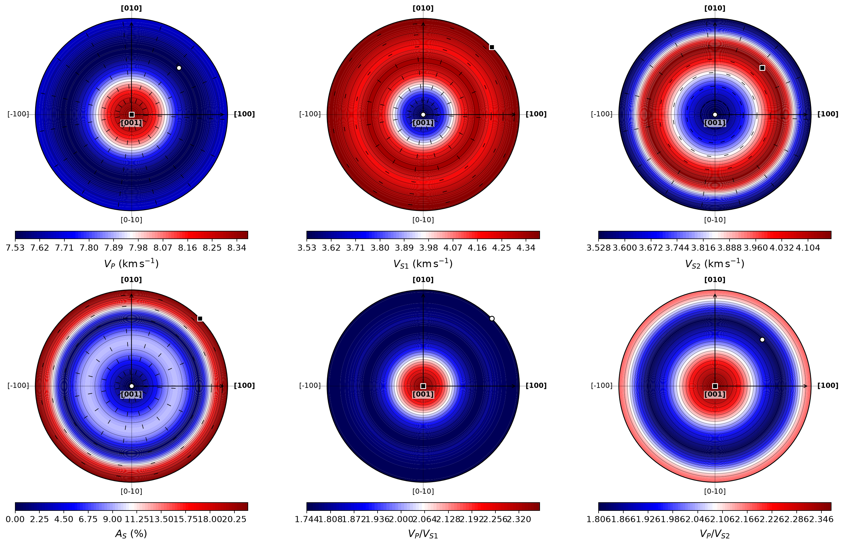
Equal-area upper-hemisphere summary of \(V_P\), \(V_{S1}\), and \(V_{S2}\), directional shear anisotropy, and the two directional \(V_P/V_S\) ratios. Minimum and maximum markers are selected from the sampled grid. Decimated black segments show tracked polarization axes on maps where they are defined.

The summary makes the hexagonal pattern immediately visible. The central point is \([001]\); the outer boundary is the basal plane. The compressional wave is fastest along \([001]\), while the largest shear splitting occurs toward the edge of the projection.

A single shear map with polarization

quantas seismic plot hydroxylapatite_seismic.hdf5 \
    --2d \
    --property phase_v_s1 \
    --projection equal_area \
    --polarization \
    --polarization-stride 8 \
    --axis-labels crystal \
    --preset publication \
    --dpi 180 \
    --output hydroxylapatite_vs1

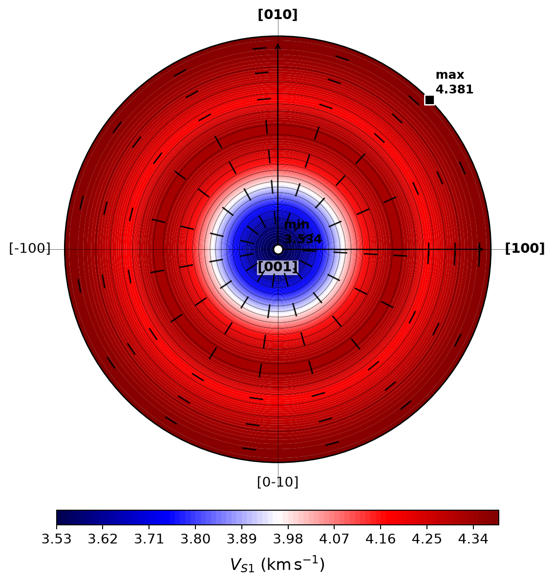
Fast shear-wave phase velocity \(V_{S1}\). The central minimum is the shear degeneracy on \([001]\); the fast branch reaches its maximum near the basal plane. Polarization segments are axial, not directed arrows, and should not be interpreted inside unresolved degenerate points.

Three-dimensional compressional phase surface

quantas seismic plot hydroxylapatite_seismic.hdf5 \
    --3d \
    --surface phase \
    --mode v_p \
    --geometry physical \
    --axis-labels crystal \
    --no-polarization \
    --preset publication \
    --dpi 180 \
    --output hydroxylapatite_vp_surface

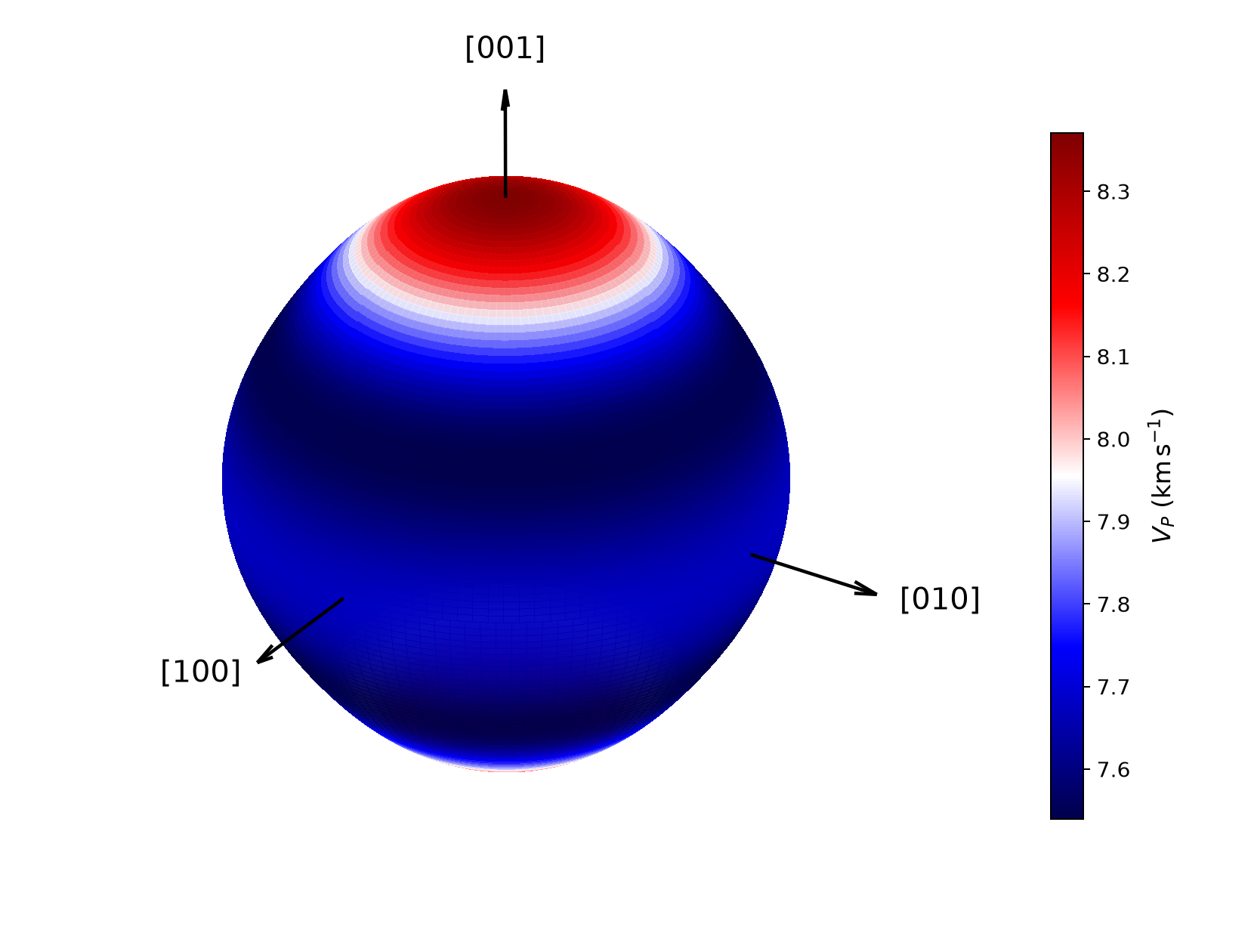
Physical \(V_P\) surface completed by antipodal symmetry from the sampled upper hemisphere. Radius and color both encode phase speed. The elongation along \([001]\) reflects the maximum compressional velocity in that direction.

The slowness and group surface types answer different questions. Slowness geometry is especially useful for wave-normal constructions, whereas the group surface represents energy-flow wavefronts.

Running the same workflow from Python

The complete public-API script is distributed with the examples:

Download the SEISMIC API script

"""Reproduce the Hydroxylapatite SEISMIC tutorial with the public API."""

from __future__ import annotations

import argparse
from pathlib import Path

import numpy as np

from quantas.api import common, rendering, seismic


def main() -> None:
    """Run SEISMIC, persist fields, export CSV, and render selected figures."""
    parser = argparse.ArgumentParser()
    parser.add_argument("input", type=Path)
    parser.add_argument(
        "--output-dir",
        type=Path,
        default=Path("seismic_tutorial"),
    )
    args = parser.parse_args()

    args.output_dir.mkdir(parents=True, exist_ok=True)

    options = seismic.Options(
        ntheta=61,
        nphi=121,
        hemisphere="upper",
        level="enhancement",
        track_polarization_axes=True,
    )
    result = seismic.run(args.input, options=options)
    payload = seismic.get_result(result)

    report = rendering.render_tables(
        seismic.build_report(result, level="extended")
    )
    report_path = args.output_dir / "hydroxylapatite_seismic_api.log"
    report_path.write_text(report, encoding="utf-8", newline="\n")
    hdf5_path = seismic.write_result(
        result,
        args.output_dir / "hydroxylapatite_seismic_api.hdf5",
        report_text=report,
    )
    csv_path = seismic.write_csv(
        result,
        args.output_dir / "hydroxylapatite_seismic_api.csv",
    )

    summary_options = seismic.PlotOptions(
        include_polarizations=True,
        polarization_stride=8,
    )
    summary = seismic.build_summary(result, options=summary_options)
    rendering.render_plots(
        common.PlotCollection(plots=[summary]),
        output_dir=args.output_dir,
        filename_prefix="hydroxylapatite_",
        preset="publication",
        dpi=180,
        close=True,
        axis_label_mode="crystal",
    )

    vs1_map = seismic.build_plots(
        result,
        seismic.PlotOptions(
            properties=("phase_v_s1",),
            projection="equal_area",
            include_extrema_markers=True,
            include_polarizations=True,
            polarization_stride=8,
        ),
    )
    rendering.render_plots(
        vs1_map,
        output_dir=args.output_dir,
        filename_prefix="hydroxylapatite_",
        preset="publication",
        dpi=180,
        close=True,
        axis_label_mode="crystal",
    )

    vp_surface = seismic.build_surfaces(
        result,
        seismic.SurfaceOptions(
            properties=(),
            modes=("v_p",),
            surface_types=("phase",),
            geometry="physical",
            include_polarizations=False,
        ),
    )
    rendering.render_plots(
        vp_surface,
        output_dir=args.output_dir,
        filename_prefix="hydroxylapatite_",
        preset="publication",
        dpi=180,
        close=True,
        axis_label_mode="crystal",
    )

    phase = payload.field.phase
    vp = phase.for_mode("v_p")
    vs1 = phase.for_mode("v_s1")
    vs2 = phase.for_mode("v_s2")
    print(f"Sampled directions: {phase.n_points}")
    print(f"Isotropic V_S / km s^-1: {payload.isotropic_velocities.shear:.8f}")
    print(
        "Isotropic V_P / km s^-1: "
        f"{payload.isotropic_velocities.compressional:.8f}"
    )
    print(f"V_P range / km s^-1: {np.nanmin(vp.phase_speeds):.8f} "
          f"{np.nanmax(vp.phase_speeds):.8f}")
    print(f"V_S1 range / km s^-1: {np.nanmin(vs1.phase_speeds):.8f} "
          f"{np.nanmax(vs1.phase_speeds):.8f}")
    print(f"V_S2 range / km s^-1: {np.nanmin(vs2.phase_speeds):.8f} "
          f"{np.nanmax(vs2.phase_speeds):.8f}")
    print(f"Written: {hdf5_path}")
    print(f"Written: {report_path}")
    print(f"Written: {csv_path}")


if __name__ == "__main__":
    main()

Run it with:

python examples/seismic/tutorial_api.py \
    examples/elasticity/hydroxylapatite.dat \
    --output-dir seismic_tutorial

The script uses only supported public namespaces:

from quantas.api import common, rendering, seismic

It demonstrates:

• construction of quantas.api.seismic.Options;

• typed access through quantas.api.seismic.get_result();

• HDF5 and CSV export;

• an extended deterministic report;

• a summary specification wrapped in a public PlotCollection;

• a selected map with polarization axes;

• a physical phase-velocity surface.

The printed checkpoints are:

Sampled directions: 7381
Isotropic V_S / km s^-1: 4.00911178
Isotropic V_P / km s^-1: 7.64303712
V_P range / km s^-1: 7.53989166 8.37032277
V_S1 range / km s^-1: 3.53384250 4.38141779
V_S2 range / km s^-1: 3.53384250 4.16716850

Inspecting structured fields

from quantas.api import seismic

result = seismic.read_result("hydroxylapatite_seismic.hdf5")
payload = seismic.get_result(result)

phase = payload.field.phase
vp = phase.for_mode("v_p")
vs1 = phase.for_mode("v_s1")

print(phase.n_points)
print(vp.phase_speeds.shape)
print(vs1.polarizations.shape)
print(phase.shear_axis_candidate_mask.sum())

if payload.field.group is not None:
    group_vp = payload.field.group.for_mode("v_p")
    print(group_vp.group_speeds.shape)
    print(group_vp.power_flow_angles.shape)

if payload.field.enhancement is not None:
    print(payload.field.enhancement.log10_enhancement.shape)
    print(payload.field.enhancement.caustic_candidate_mask.sum())

All arrays use the same ordered spherical grid. Masks must be respected when working with degenerate or unresolved quantities.

CLI/API equivalence

import numpy as np
from quantas.api import seismic

cli = seismic.get_result(
    seismic.read_result("hydroxylapatite_seismic.hdf5")
)
api = seismic.get_result(
    seismic.read_result(
        "seismic_tutorial/hydroxylapatite_seismic_api.hdf5"
    )
)

np.testing.assert_allclose(
    cli.field.phase.phase_speeds,
    api.field.phase.phase_speeds,
)
np.testing.assert_allclose(
    cli.field.group.group_speeds,
    api.field.group.group_speeds,
    equal_nan=True,
)
np.testing.assert_allclose(
    cli.field.enhancement.log10_enhancement,
    api.field.enhancement.log10_enhancement,
    equal_nan=True,
)

Reproducibility checkpoints

For the documented grid and default numerical tolerances:

Quantity	Expected value
Elastic symmetry	hexagonal
Sampled directions	7381
Isotropic \(V_S\) / km s⁻¹	4.00911178
Isotropic \(V_P\) / km s⁻¹	7.64303712
Minimum \(V_P\) / km s⁻¹	7.53989166
Maximum \(V_P\) / km s⁻¹	8.37032277
Maximum shear splitting / km s⁻¹	0.84757530
Maximum directional shear anisotropy / %	21.41623306
Caustic candidates on this grid	0

The phase speeds at a fixed sampled direction should be invariant to batch size. Sampled extrema, equivalent-point counts, and possible caustic detection can change when angular resolution or numerical tolerances are changed.

Grid-convergence exercise

Repeat the calculation with a denser grid:

quantas seismic run examples/elasticity/hydroxylapatite.dat \
    --hemisphere upper \
    --level enhancement \
    --ntheta 121 \
    --nphi 241 \
    --output hydroxylapatite_seismic_dense.hdf5 \
    --report hydroxylapatite_seismic_dense.log \
    --no-progress \
    --force

Compare:

• phase-velocity minima and maxima;

• maximum shear splitting;

• number and location of shear-axis candidate points;

• extrema of \(\log_{10}(A)\);

• caustic-candidate count.

Phase fields generally converge more smoothly than enhancement fields because enhancement depends on curvature. A candidate that appears only on one coarse grid should be treated as a numerical hypothesis requiring refinement, not as a confirmed physical caustic.