P–V–T tutorial: coupled EOS of NaF

Scientific objective

A P–V–T dataset samples several temperatures and pressures simultaneously. The goal is not only to fit compression and expansion, but to choose a coupling that describes how the zero-pressure reference state and elastic response vary with temperature.

The curated NaF dataset contains 48 observations from 140 to 350 K and up to a few gigapascals. It declares:

VSCALE cm^3/mol
format: T, sigT, P, sigP, V, sigV

The volume is molar volume per formula unit. This matters for Mie–Grüneisen– Debye normalization: the formula NaF represents two atoms per molar formula unit.

Why use the batch specification here?

P–V–T models are compositions of several scientific choices. The supplied specification makes those choices explicit and compares four couplings:

BM3 + quadratic Berman + linear \(K_0(T)\);
BM3 + quadratic Berman + Anderson–Grüneisen coupling;
BM3 + Holland–Powell Einstein thermal pressure;
BM4 + full Mie–Grüneisen–Debye thermal pressure.

Validate and run:

quantas eos run examples/eos/PVT_NaF.dat \
    --spec examples/eos/specs/naf_pvt_tutorial.spec \
    --dry-run

quantas eos run examples/eos/PVT_NaF.dat \
    --spec examples/eos/specs/naf_pvt_tutorial.spec \
    --output naf_pvt.hdf5 \
    --report naf_pvt.log \
    --verbosity extended \
    --force

All four records are retained; the full-MGD record is accepted for post-fit examples.

Parameter constraints in the MGD job

The reference temperature is fixed:

fix.temperature_ref = 295.0

The thermal parameters are free but physically bounded:

initial.theta_d0 = 459.0
bound.theta_d0 = 1.0 : 5000.0
initial.gamma0 = 1.5
bound.gamma0 = 0.01 : 10.0
initial.q = 1.0
bound.q = -10.0 : 10.0

The normalization is explicit:

volume_basis = molar-formula-unit
formula = NaF

Bounds are not a substitute for information in the data. A parameter that is strongly correlated or weakly resolved should be fixed from an independent source or reported cautiously.

Coupling comparison

The full generated table is available as naf_pvt_coupling_comparison.csv.

Coupling	\(K_0\) (GPa)	\(K'_0\)	\(V_0\)	\(V(1.5\,\mathrm{GPa},230\,\mathrm K)\)	\(\alpha(1.5\,\mathrm{GPa},230\,\mathrm K)\)	RMSE (GPa)
Linear \(K_0(T)\)	44.868125	6.720167	14.974354	14.453937	6.840725e−5	0.028589
Anderson–Grüneisen	44.900978	6.745525	14.974230	14.454340	6.877433e−5	0.028091
HP Einstein thermal pressure	44.813167	7.023415	14.974418	14.453650	7.149799e−5	0.034077
Full MGD	45.339416	6.149515	14.969663	14.454408	6.995470e−5	0.029156

The predicted volume at an interior state is very similar for all models, even though the reference elastic parameters differ. The data therefore constrain interpolation more tightly than they uniquely identify a coupling model.

Full-MGD result

V0       = 14.969663 ± 0.002184 cm³ mol⁻¹
K0       = 45.339416 ± 0.966802 GPa
K′       =  6.149515 ± 1.413508
K″       =  0.117985 ± 0.926164 GPa⁻¹
theta_D0 = 523.146380 ± 52.021961 K
gamma0   =  1.624893 ± 0.071257
q        =  2.040148 ± 0.788557

RMSE                 = 0.029156 GPa
reduced chi-square   = 2.802172

The large uncertainty in \(K''_0\) and the substantial uncertainties in \(K'_0\) and \(q\) must be reported. The fit is useful, but the dataset does not determine every curvature parameter with equal precision.

Pressure–temperature coverage

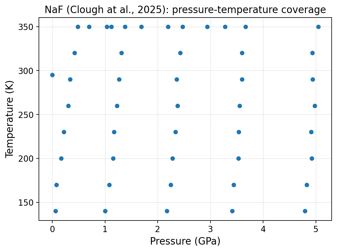
Coverage is not a rectangular grid. Before interpreting a P–V–T surface, identify where observations actually constrain it. A calculated state inside the bounding box may still be distant from measured combinations of pressure and temperature.

Isotherms

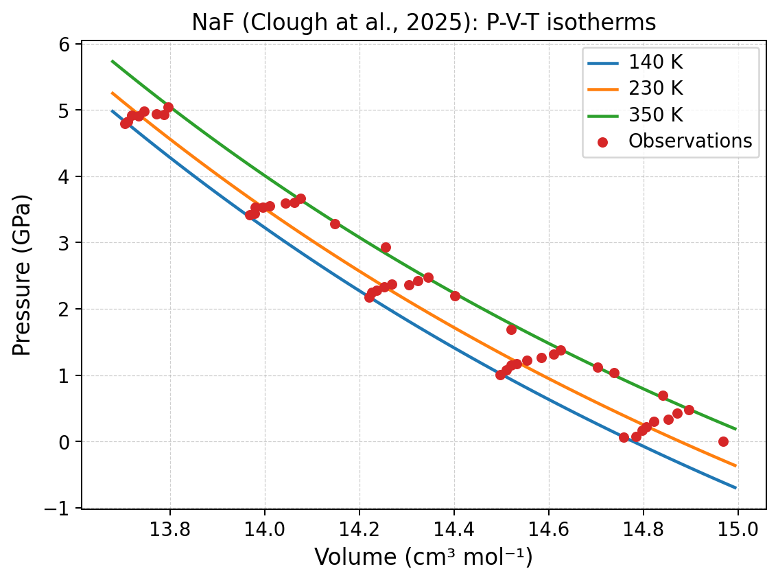
The isotherms shift to larger volume with increasing temperature. Their spacing and curvature reflect both thermal pressure and the volume dependence of the cold compression curve.

Generate them with:

quantas eos plot naf_pvt.hdf5 --slot pvt/volume \
    --plot isotherms \
    --isotherm 140 --isotherm 230 --isotherm 350 \
    --curve-points 60 \
    --preset publication \
    --output naf_isotherms

Isobars

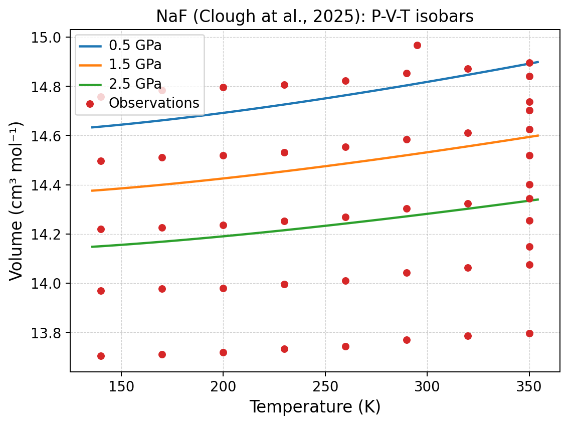
Higher pressure lowers the volume and changes the thermal-expansion response. The nearly parallel curves over this restricted range do not imply that the coupling remains linear outside it.

Residuals

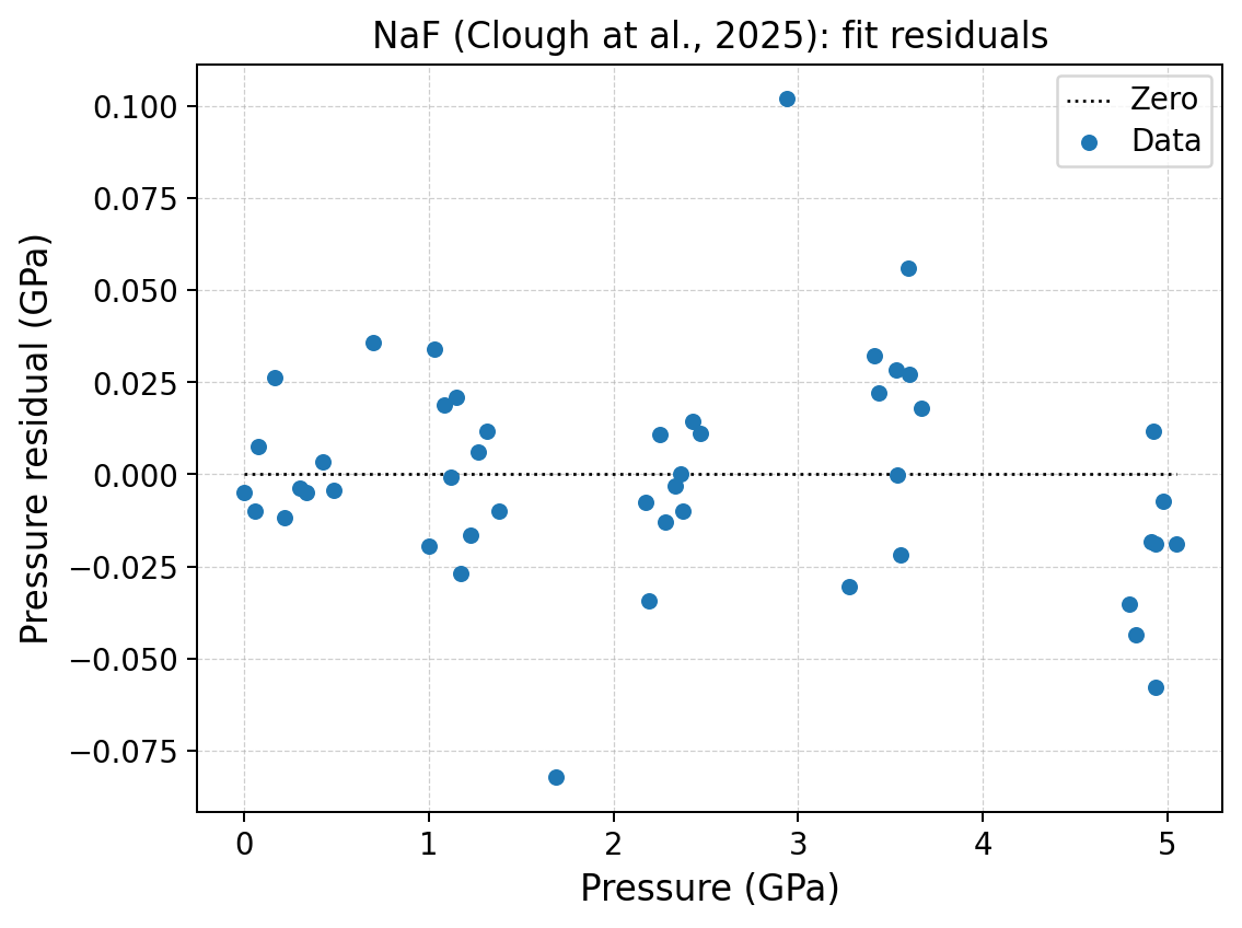
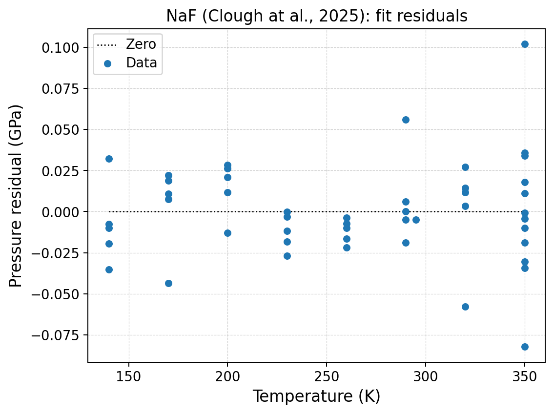
Both projections are necessary. A pattern invisible against pressure may be obvious against temperature, and vice versa. Residual plots should be read together with parameter correlations and the P–T coverage.

Post-fit property calculation

Evaluate a Cartesian state grid:

quantas eos calculate naf_pvt.hdf5 --slot pvt/volume \
    --pressure-range 0.5:2.5:0.5 \
    --temperature-range 140:350:30 \
    --output naf_pvt_properties.csv

The result includes volume, \(K_T\), its pressure derivatives, \(\alpha(P,T)\), \((\partial K/\partial T)_P\), thermal pressure where available, propagated parameter uncertainty, and extrapolation flags.

Python API

Download pvt_fit_api.py

"""Fit the NaF P-V-T example with a full Mie-Gruneisen-Debye model."""

from __future__ import annotations

from pathlib import Path

from quantas.api import eos

ROOT = Path(__file__).resolve().parents[1]
DATA = ROOT / "PVT_NaF.dat"


def main() -> None:
    """Run the public volume-only MGD fit using molar-volume normalization."""
    dataset = eos.read_input(DATA)
    normalization = eos.MGDNormalization.molar_formula_unit(formula="NaF")
    model = eos.PVTModel(
        pressure_model="BM4",
        coupling="thermal-pressure",
        thermal_pressure_model="mgd",
        mgd_normalization=normalization,
    )
    constraints = (
        eos.ParameterConstraint.fixed("temperature_ref", 295.0),
        eos.ParameterConstraint.free(
            "theta_d0", 459.0, lower_bound=1.0, upper_bound=5000.0
        ),
        eos.ParameterConstraint.free(
            "gamma0", 1.5, lower_bound=0.01, upper_bound=10.0
        ),
        eos.ParameterConstraint.free(
            "q", 1.0, lower_bound=-10.0, upper_bound=10.0
        ),
    )
    request = eos.FitRequest(
        model=model,
        domain="pvt",
        target="volume",
        constraints=constraints,
        options=eos.FitOptions(
            solver_options=eos.EffectiveVarianceOptions(
                max_iterations=50,
                inner_max_iterations=10000,
            )
        ),
        request_id="naf-bm4-mgd-effective-variance",
    )
    result = eos.fit(dataset, request)
    if not result.fit.success:
        raise RuntimeError(result.fit.message)

    print("NaF BM4 + full-MGD effective-variance fit")
    print("==========================================")
    for name in ("V0", "K0", "KP", "KPP", "theta_d0", "gamma0", "q"):
        print(f"{name:10s} = {result.parameter_values[name]:.10g}")
    print(f"RMSE       = {result.fit.rmse:.10g} GPa")


if __name__ == "__main__":
    main()

The script uses molar-formula-unit MGD normalization, matching the volume unit declared by the input file.

Exercise 1: release fewer parameters

Repeat the MGD fit with \(\theta_{D0}=459\) K and \(q=1\) fixed, leaving only \(\gamma_0\) free among the thermal parameters.

Fit	Free thermal parameters	\(K_0\)	\(K'_0\)	\(\gamma_0\)	RMSE	Largest correlation
Full MGD	\(\theta_{D0},\gamma_0,q\)	45.339416	6.149515	1.624893	0.029156	`inspect report`
Controlled MGD	\(\gamma_0\)	`...`	`...`	`...`	`...`	`...`

Discuss the trade-off between a slightly less flexible fit and more stable, externally constrained parameters.

Exercise 2: compare outside the dense data region

Calculate each coupling at 0.5 GPa and 140 K, at 1.5 GPa and 230 K, and at 2.5 GPa and 350 K. Then add one state outside the observed temperature range. Complete:

Coupling	Interior volume	Interior \(K_T\)	Interior \(\alpha\)	Extrapolated volume	Extrapolation flag
Linear	14.453937	56.846399	6.840725e−5	`...`	`...`
Anderson–Grüneisen	14.454340	57.015775	6.877433e−5	`...`	`...`
HP Einstein	14.453650	56.933508	7.149799e−5	`...`	`...`
Full MGD	14.454408	56.853635	6.995470e−5	`...`	`...`

The divergence outside the measured domain is more informative about model assumptions than the near-equality of interpolated volumes.