P–V tutorial: quartz compression

Scientific objective

This tutorial determines the reference volume, bulk modulus, and pressure derivative of quartz from an isothermal compression dataset. It also shows how model order and uncertainty treatment affect the inferred parameters.

The curated file is:

examples/eos/PV_quartz.dat

It contains 22 observations from approximately 0 to 8.9 GPa, with standard uncertainties for both pressure and volume.

Inspecting the input

The header declares the column order:

format 1 P V SigP SigV

and the first observations are:

0.000  112.981   1.000E-6  0.002
0.430  111.725   0.008     0.014
0.794  110.711   0.008     0.006

The zero-pressure point strongly constrains \(V_0\). Its tiny pressure uncertainty also makes the distinction between WLS and coordinate-aware methods particularly visible.

A single direct fit

Run a third-order Birch–Murnaghan fit with effective variance:

quantas eos run examples/eos/PV_quartz.dat \
    --domain pv \
    --fit volume \
    --pv-eos birch-murnaghan \
    --pv-order 3 \
    --solver effective-variance \
    --max-iterations 50 \
    --inner-max-iterations 10000 \
    --show-uncertainties \
    --verbosity extended \
    --output quartz_bm3_ev.hdf5 \
    --report quartz_bm3_ev.log \
    --force

The principal result is:

V0   = 112.980884 ± 0.001993 ų
K0   =  37.125926 ± 0.091051 GPa
K′   =   5.988260 ± 0.045302
K″   =  -0.264783 ± 0.006703 GPa⁻¹  [implied]

RMSE                 = 0.011133 GPa
reduced chi-square   = 0.952062
selected observations = 22

The third-order model has three free parameters: \(V_0\), \(K_0\), and \(K'_0\). The reported \(K''_0\) is implied by the selected EOS and must not be interpreted as a fourth independently fitted parameter.

Running the comparison batch

The supplied specification performs three solver comparisons and three model comparisons:

quantas eos run examples/eos/PV_quartz.dat \
    --spec examples/eos/specs/quartz_pv_tutorial.spec \
    --dry-run

quantas eos run examples/eos/PV_quartz.dat \
    --spec examples/eos/specs/quartz_pv_tutorial.spec \
    --output quartz_pv.hdf5 \
    --report quartz_pv.log \
    --verbosity extended \
    --force

The complete generated comparison is available as quartz_pv_comparison.csv.

Solver comparison

Solver	\(V_0\) (ų)	\(K_0\) (GPa)	\(K'_0\)	RMSE (GPa)	Reduced \(\chi^2\)
OLS	112.967525	37.285421	5.933527	0.010898	—
WLS	112.981000	37.145494	5.976661	0.011033	1.571859
Effective variance	112.980884	37.125926	5.988260	0.011133	0.952062

The RMSE values are similar because all three methods describe the same smooth curve. The parameters nevertheless shift because the objective functions are different. OLS does not use the precision information. WLS gives very high weight to the near-zero-pressure observation through \(\sigma_P\) but does not project \(\sigma_V\). Effective variance includes both uncertainty components.

Model-order comparison

Keeping effective variance fixed isolates the effect of the EOS formulation:

Model	\(V_0\) (ų)	\(K_0\) (GPa)	\(K'_0\)	RMSE (GPa)	Reduced \(\chi^2\)
BM2	112.968349	41.475671	4.000000 fixed	0.133695	128.265150
BM3	112.980884	37.125926	5.988260	0.011133	0.952062
PT3	112.981299	36.396317	6.909770	0.012001	1.156613
V3	112.980947	37.025430	6.103146	0.010795	0.902934

BM2 is clearly too restrictive for this dataset: fixing \(K'_0=4\) forces \(K_0\) upward and leaves large systematic residuals. BM3 and V3 agree closely in \(V_0\) and \(K_0\), while PT3 requires a larger \(K'_0\). Agreement in RMSE alone is not enough to claim that the parameters of different functional forms are interchangeable.

Fit and residual figures

Generate the accepted BM3 figures with:

quantas eos plot quartz_pv.hdf5 --slot pv/volume \
    --plot fit --plot residuals --plot normalized-pressure \
    --preset publication --format png --dpi 180 \
    --output quartz_pv_plots

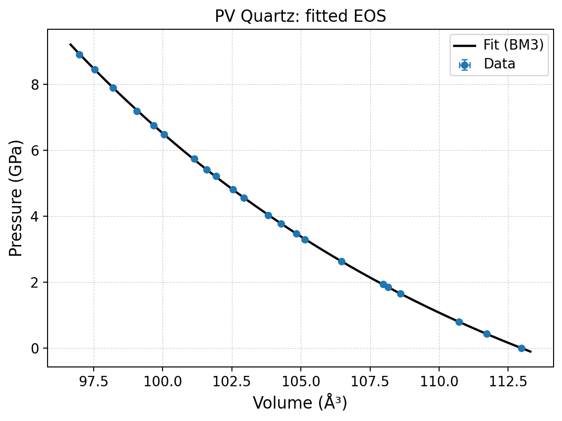
At the scale of the full compression curve, the fit appears almost exact. The residual panel is therefore essential:

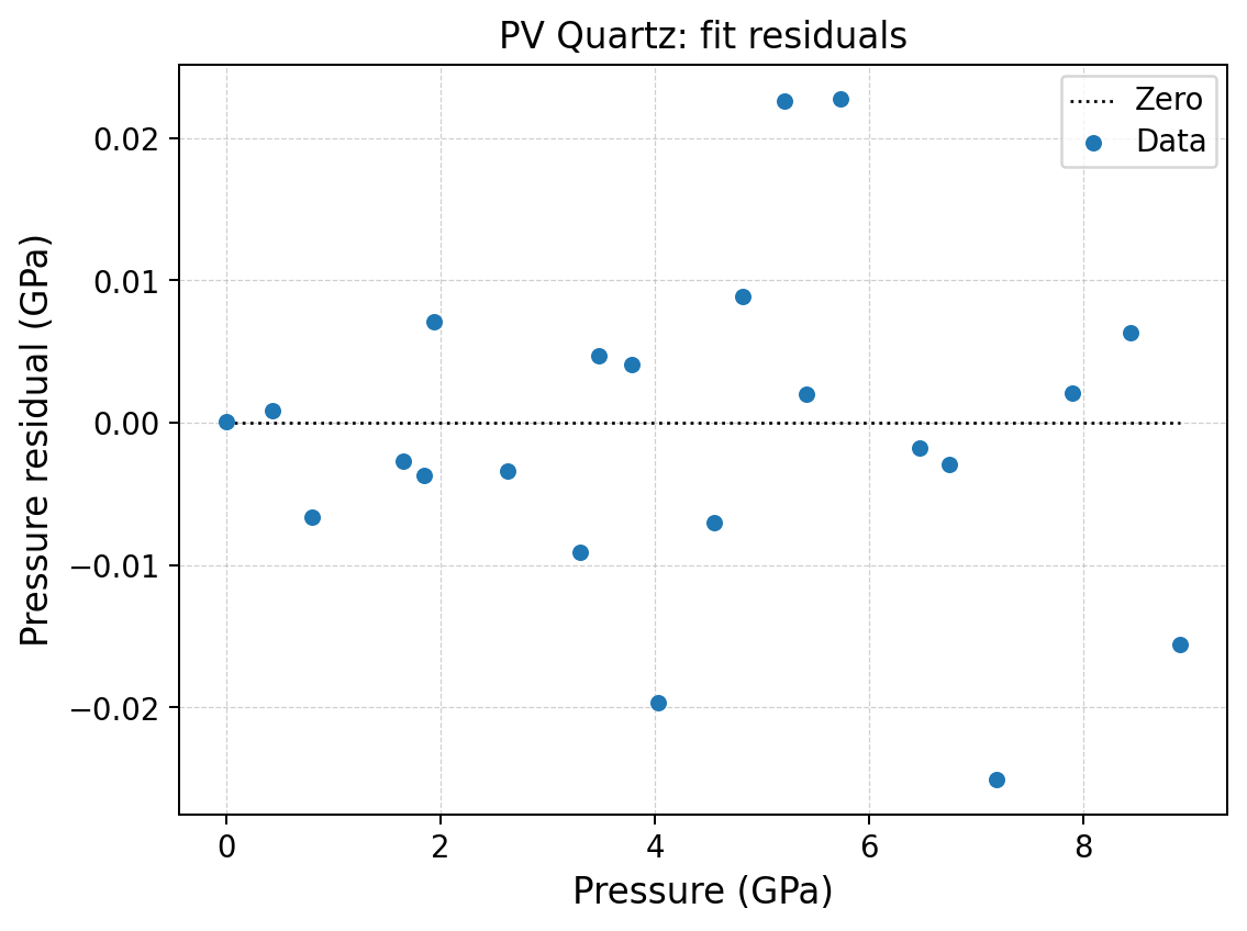
The residuals fluctuate around zero without the strong curvature seen in the BM2 fit. Individual points near 4, 5.2, 5.7, and 7.2 GPa deserve attention, but no single observation controls the entire curve.

Normalized-pressure diagnostic

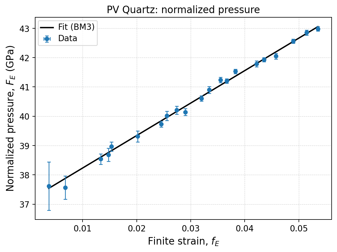
For Birch–Murnaghan, the \(F_E-f_E\) representation is a model-order diagnostic. A non-zero slope indicates that BM2 is inadequate. The exact zero-pressure point is hidden by default because normalized pressure is singular at zero strain; the observation remains part of the fit and archive.

Post-fit calculation

Calculate volumes and moduli without refitting:

quantas eos calculate quartz_pv.hdf5 --slot pv/volume \
    --pressure-range 0:10:1 \
    --output quartz_pv_properties.csv

Values above the maximum measured pressure are flagged as extrapolated. A smooth EOS curve does not remove the scientific uncertainty of extrapolation.

Python API

Download pv_fit_api.py

"""Fit the quartz P-V example with BM3 effective variance."""

from __future__ import annotations

from pathlib import Path

from quantas.api import eos

ROOT = Path(__file__).resolve().parents[1]
DATA = ROOT / "PV_quartz.dat"


def main() -> None:
    """Run one public P-V request and print the principal results."""
    dataset = eos.read_input(DATA)
    request = eos.FitRequest(
        model="BM3",
        domain="pv",
        target="volume",
        options=eos.FitOptions(
            solver_options=eos.EffectiveVarianceOptions(
                max_iterations=50,
                inner_max_iterations=10000,
            )
        ),
        request_id="quartz-bm3-effective-variance",
    )
    result = eos.fit(dataset, request)
    if not result.fit.success:
        raise RuntimeError(result.fit.message)

    print("Quartz BM3 effective-variance fit")
    print("=================================")
    for name in ("V0", "K0", "KP", "KPP"):
        print(f"{name:4s} = {result.parameter_values[name]:.9g}")
    print(f"RMSE = {result.fit.rmse:.8f} GPa")
    diagnostics = result.fit.diagnostics
    if diagnostics is not None:
        print(f"Reduced chi-square = {diagnostics.reduced_chi_square:.8f}")


if __name__ == "__main__":
    main()

Exercise 1: is BM4 justified?

Add an effective-variance BM4 job. Record \(K''_0\), its E.S.D., the largest parameter correlations, RMSE, and reduced chi-square.

Model	\(K_0\)	\(K'_0\)	\(K''_0\)	E.S.D. of \(K''_0\)	Reduced \(\chi^2\)
BM3	37.125926	5.988260	−0.264783 implied	0.006703 propagated	0.952062
BM4	...	...	...	...	...

A fourth-order model is justified only if the additional independent curvature is resolved and scientifically stable, not merely because RMSE decreases.

Exercise 2: axial compression of topaz

Repeat the workflow with PV_topaz.dat and targets = volume, a, b, c. Compare the axial moduli and remember that Quantas fits the auxiliary cubed length while reporting physical lengths and linear moduli.