V–T tutorial: thermal expansion of rutile

Scientific objective

The rutile dataset collects relative unit-cell volume and axial lengths over a broad temperature interval at approximately constant pressure. The tutorial fits the volumetric expansion, compares solver assumptions and thermal models, and then resolves the anisotropic expansion of the a and c axes.

Input conventions

The file declares:

SYSTEM tetragonal
TSCALE K
VSCALE V/V0
LSCALE L/L0
format: T, sigT, P, sigP, V, sigV, a, siga, c, sigc

The normalized values are dimensionless. Consequently the fitted reference V0 is a scale factor close to one, not an absolute crystallographic volume in ų.

The pressure is nearly constant, so the dataset is accepted as isobaric. A V–T fit would be scientifically invalid if pressure varied enough to produce a significant compression signal.

Direct CLI fit

quantas eos run examples/eos/VT_rutile.dat \
    --domain vt \
    --fit volume \
    --vt-eos berman \
    --vt-variant quadratic \
    --solver effective-variance \
    --max-iterations 30 \
    --inner-max-iterations 5000 \
    --show-uncertainties \
    --verbosity extended \
    --output rutile_berman_ev.hdf5 \
    --report rutile_berman_ev.log \
    --force

The accepted result is:

V0      = 1.000576906 ± 0.000071542
Tref    = 298.15 K  [fixed]
alpha0  = 2.178651e-05 ± 3.881976e-07 K^-1
alpha1  = 2.031522e-08 ± 1.542115e-09 K^-2

RMSE                 = 6.49548e-04
reduced chi-square   = 8.10868

The reduced chi-square substantially exceeds one. With inflate-only covariance scaling, the fitted minimum is unchanged but the reported parameter errors are enlarged. This is a warning that scatter between literature groups is larger than implied by the supplied standard uncertainties.

Batch comparison

quantas eos run examples/eos/VT_rutile.dat \
    --spec examples/eos/specs/rutile_vt_tutorial.spec \
    --output rutile_vt.hdf5 \
    --report rutile_vt.log \
    --verbosity extended \
    --force

Download the full table: rutile_vt_comparison.csv.

Solver sensitivity

For the same quadratic Berman model:

Solver	\(V_0\)	\(\alpha(300\,\mathrm K)\)	\(\alpha(1000\,\mathrm K)\)	RMSE	Reduced \(\chi^2\)
OLS	1.000387868	2.288707e−5	3.319814e−5	5.95657e−4	—
WLS	1.000540118	2.195726e−5	3.602436e−5	6.86642e−4	13.742329
Effective variance	1.000576906	2.182321e−5	3.532779e−5	6.49548e−4	8.108683

The three fits are visually similar but differ in the inferred high-temperature expansion. Temperature uncertainty matters because the derivative \(dV/dT\) is the quantity of interest.

Thermal-model sensitivity

At fixed effective variance:

Model	\(V_0\)	\(\alpha(300\,\mathrm K)\)	\(\alpha(1000\,\mathrm K)\)	RMSE	Reduced \(\chi^2\)
Berman quadratic	1.000576906	2.182321e−5	3.532779e−5	6.49548e−4	8.108683
Fei inverse-square	1.000027989	2.683717e−5	3.022912e−5	6.48632e−4	4.106359
Salje	0.995585814	2.623640e−5	2.932552e−5	6.40656e−4	3.781740

All three reproduce the measured range with similar RMSE, but their reference parameters and extrapolated expansion differ. This is the central lesson of a V–T model comparison: fit quality inside the sampled interval does not make low- or high-temperature extrapolations equivalent.

Fit and residual plots

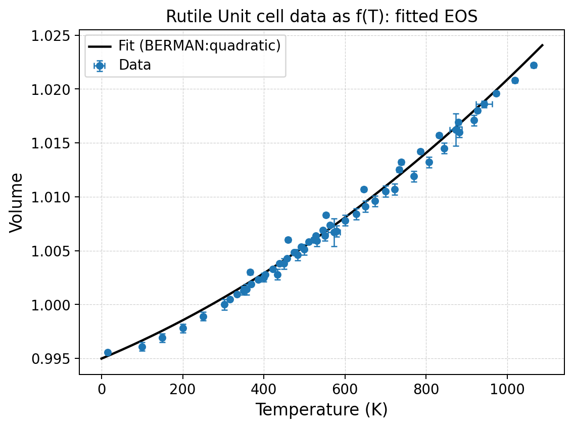
The full curve is smooth and the different literature groups overlap closely. The residual plot reveals the remaining structure:

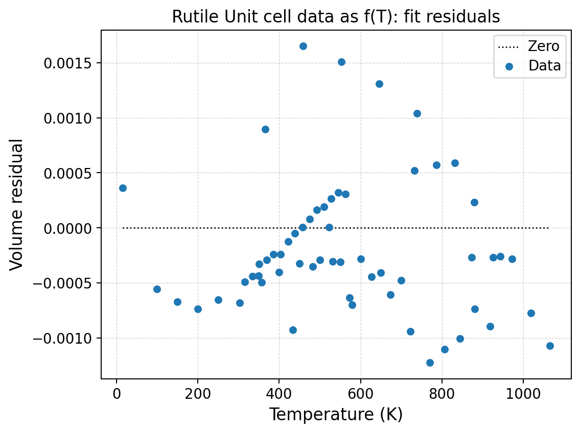
Systematic offsets between groups are more scientifically informative than the small absolute scale of the residuals.

The plotting path also enforces the physical lower bound on temperature: curve padding is clipped above zero kelvin rather than evaluating the thermal model at negative temperature.

Axial thermal expansion

The specification also fits the tetragonal a and c axes. Quantas uses the same cubed-length convention as EosFit and converts results back to physical lengths and linear expansion coefficients.

a axis:
    L0      = 1.000161205
    alpha0  = 1.976343e-05 K^-1
    alpha1  = 1.911215e-08 K^-2

c axis:
    L0      = 1.000203045
    alpha0  = 2.478942e-05 K^-1
    alpha1  = 3.482191e-08 K^-2

The c direction expands more strongly than a in this model. For a tetragonal cell, the volumetric response is related to the two linear responses, but independently fitted noisy datasets need not satisfy the identity exactly.

Post-fit calculation

quantas eos calculate rutile_vt.hdf5 --slot vt/volume \
    --temperature-range 300:1100:100 \
    --output rutile_thermal_properties.csv

The output includes fitted volume, expansion coefficient, temperature derivative, propagated parameter uncertainty, and extrapolation flags.

Python API

Download vt_fit_api.py

"""Fit the rutile V-T example with the quadratic Berman model."""

from __future__ import annotations

from pathlib import Path

from quantas.api import eos

ROOT = Path(__file__).resolve().parents[1]
DATA = ROOT / "VT_rutile.dat"


def main() -> None:
    """Run one public V-T request and calculate representative states."""
    dataset = eos.read_input(DATA)
    request = eos.FitRequest(
        model="berman:quadratic",
        domain="vt",
        target="volume",
        options=eos.FitOptions(
            solver_options=eos.EffectiveVarianceOptions(
                max_iterations=30,
                inner_max_iterations=5000,
            )
        ),
        request_id="rutile-berman-effective-variance",
    )
    result = eos.fit(dataset, request)
    if not result.fit.success:
        raise RuntimeError(result.fit.message)

    print("Rutile quadratic-Berman effective-variance fit")
    print("================================================")
    for name in ("V0", "temperature_ref", "alpha0", "alpha1"):
        print(f"{name:16s} = {result.parameter_values[name]:.10g}")
    print(f"RMSE             = {result.fit.rmse:.10g}")


if __name__ == "__main__":
    main()

Exercise 1: complete the ODR row

Add a Berman quadratic ODR job and complete:

Solver	\(V_0\)	\(\alpha_0\)	\(\alpha_1\)	RMSE	Strongest correlation
Effective variance	1.000576906	2.178651e−5	2.031522e−8	6.49548e−4	inspect report
ODR	...	...	...	...	...

Explain whether the differences arise from model physics or from the regression objective.

Exercise 2: test extrapolation

Calculate \(\alpha(T)\) at 50, 300, 1000, and 1500 K for Berman, Fei, and Salje records. Mark which states lie outside the sampled temperature interval. Do not rank the models from extrapolated values alone; compare their limiting assumptions in the scientific-background chapter.