Quasi-Harmonic Approximation
This tutorial extends the MgO harmonic calculation to finite pressure and temperature. Quantas fits the volume dependence of the static and vibrational contributions, minimizes the appropriate thermodynamic potential, and produces equilibrium structural and thermodynamic properties on a pressure-temperature grid.
Scientific objective
For temperatures from 0 to 1000 K and pressures from 0 to 10 GPa, calculate:
equilibrium volume, \(V(P,T)\);
isothermal and adiabatic bulk moduli, \(K_T\) and \(K_S\);
volumetric and axial thermal expansion;
\(C_V\), \(C_P\), and \(C_P-C_V\);
thermodynamic and mode-weighted Grüneisen parameters;
equilibrium lattice parameters.
Dataset and relationship to HA
The tutorial uses the same normalized MgO input as the HA tutorial:
The file can be regenerated from the distributed CRYSTAL QHA output with
quantas qha inpgen examples/qha/crystal-qha/mgo-b3lyp-crystal-qha.out \
    --interface crystal-qha \
    --jobname "MgO Periclase (CRYSTAL17 QHA)" \
    --output mgo_b3lyp.yaml
The generated YAML records mode_continuity: verified with
method: crystal-qha because the native CRYSTAL workflow explicitly reports
continuity of the frequencies with volume. This is source-managed provenance;
it is distinct from the Quantas eigenvector tracking used for independent
single-volume phonon outputs. See
Phonon input generation and mode continuity.
In HA, the eleven volumes were independent calculation points. In QHA, their static energies and phonon properties define continuous volume-dependent models. Quantas then searches these models for the equilibrium state at every requested pressure and temperature.
Inspecting the static energy-volume range
Before running QHA, inspect the pressure range represented by the static energy-volume dataset:
quantas qha inspect examples/qha/crystal-qha/mgo_b3lyp.yaml \
    --degree 3 \
    --eos BM3 \
    --report mgo_qha_inspect.log
The preview evaluates pressure from both a third-degree polynomial and a third-order Birch–Murnaghan energy EOS. Selected rows are:
    V              E             P polynomial   P EOS
  (A^3)       (Ha cell^-1)          (GPa)       (GPa)
15.495427  -2.754467055837E+02      47.20332    48.88299
18.896862  -2.754628820004E+02      -0.37565    -0.06903
21.164485  -2.754585023425E+02     -13.95094   -15.29253
The BM3 preview yields:
E0 = -275.46288 Ha cell^-1
V0 = 18.889084 A^3
K0 = 167.81087 GPa
K' = 3.897373
RMSE = 1.8692458E-06 Ha cell^-1
Quality = good
The sampled static dataset spans approximately -15 to 49 GPa according to this fit. The tutorial domain, 0–10 GPa, is therefore comfortably inside the static pressure coverage. This does not by itself guarantee that every finite-temperature equilibrium point is interpolation-only, but it is an important preliminary check.
Choosing the QHA model
This tutorial uses:
--scheme freqFit each phonon branch as a function of volume and evaluate the frequencies at the equilibrium volume. The input records verified, source-managed continuity from the native CRYSTAL QHA calculation. This is sufficient for mode-resolved QHA while preserving the actual provenance of the continuity assessment.
--minimization polyRepresent the free-energy curves by polynomials and minimize them at each pressure-temperature point.
--energy-degree 3and--frequency-degree 3Use third-degree volume fits for the static/free-energy and frequency branches.
--thermal-expansion mixed_derivativeCalculate \(\alpha_V\) from the mixed derivative of the fitted free-energy surface. The mode-Grüneisen route remains available as an internal consistency comparison.
The choices are appropriate for this dataset and tutorial. They are not universal defaults for all materials: fit quality, sampling range, branch continuity, and extrapolation must be assessed for each calculation.
Running QHA from the command line
quantas qha run examples/qha/crystal-qha/mgo_b3lyp.yaml \
    --scheme freq \
    --minimization poly \
    --thermal-expansion mixed_derivative \
    --temperature 0 1000 100 \
    --pressure 0 10 2 \
    --energy-degree 3 \
    --frequency-degree 3 \
    --output mgo_qha.hdf5 \
    --report mgo_qha.log \
    --verbosity standard \
    --no-progress \
    --force
The grid contains 11 temperatures and 6 pressures, for 66 equilibrium states. The workflow summary for this run reports:
processed points: 66
successful points: 66
warning points: 0
failed points: 0
stopped: False
Reading the QHA results
Pressure and temperature effects
Selected values at 0 GPa are:
T (K) |
V (ų) |
\(K_T\) (GPa) |
\(K_S\) (GPa) |
\(\alpha_V\) (10⁻⁵ K⁻¹) |
\(\gamma\) |
\(C_P-C_V\) (J mol⁻¹ K⁻¹) |
|---|---|---|---|---|---|---|
0 |
19.050555 |
169.13961 |
169.13961 |
0.000000 |
0.00000 |
0.0000 |
300 |
19.128633 |
163.53085 |
165.72304 |
2.933514 |
1.52324 |
0.4863 |
1000 |
19.669793 |
132.62196 |
142.54810 |
4.771473 |
1.56860 |
3.5766 |
At 10 GPa, the same temperatures give:
T (K) |
V (ų) |
\(K_T\) (GPa) |
\(K_S\) (GPa) |
\(\alpha_V\) (10⁻⁵ K⁻¹) |
\(\gamma\) |
\(C_P-C_V\) (J mol⁻¹ K⁻¹) |
|---|---|---|---|---|---|---|
0 |
18.076209 |
210.55424 |
210.55424 |
0.000000 |
0.00000 |
0.0000 |
300 |
18.126469 |
206.93427 |
208.73471 |
2.110356 |
1.37426 |
0.3018 |
1000 |
18.488160 |
188.59458 |
197.05656 |
3.187630 |
1.40759 |
2.1336 |
Several expected trends are visible:
temperature expands the cell at every pressure;
pressure compresses the cell and reduces \(\alpha_V\);
\(K_T\) decreases with temperature but increases strongly with pressure;
\(K_S\) exceeds \(K_T\) at finite temperature because \(C_P>C_V\);
the thermodynamic and mode-weighted Grüneisen parameters are close over the resolved range.
The last point is an internal consistency observation, not an independent experimental validation. For this run, the RMS difference between the two macroscopic Grüneisen estimates is approximately 0.00546.
Structural results
Because the input contains a volume-dependent structural path, Quantas also reconstructs the equilibrium cell. At 0 GPa:
   T       V          a          b          c
  (K)    (A^3)       (A)        (A)        (A)
   0   19.050555   4.239577   4.239577   4.239577
 300   19.128633   4.245361   4.245361   4.245361
1000   19.669793   4.285024   4.285024   4.285024
MgO is cubic, so \(a=b=c\) and each linear expansion coefficient equals one third of the volumetric coefficient. The report explicitly verifies that the trace of the linear expansion tensor agrees with \(\alpha_V\).
Exporting QHA tables
Equilibrium volume can be exported as CSV:
quantas qha export mgo_qha.hdf5 \
    --property VT \
    --format csv \
    --output mgo_qha_VT.csv
Download the complete equilibrium-volume CSV table
P (GPa),T (K),VT (A^3)
0.00,0.00,19.050555
0.00,300.00,19.128633
0.00,1000.00,19.669793
2.00,0.00,18.832876
2.00,300.00,18.903092
2.00,1000.00,19.390178
The expansion method is retained in a property-specific export:
quantas qha export mgo_qha.hdf5 \
    --property alphaV \
    --format csv \
    --output mgo_qha_alphaV.csv
Download the complete thermal-expansion CSV table
P (GPa),T (K),alphaV (K^-1),alphaV method
0.00,0.00,0.000000E+00,mixed_derivative
0.00,300.00,2.933514E-05,mixed_derivative
0.00,1000.00,4.771473E-05,mixed_derivative
10.00,300.00,2.110356E-05,mixed_derivative
10.00,1000.00,3.187630E-05,mixed_derivative
Generating selected QHA plots
Equilibrium volume
quantas qha plot mgo_qha.hdf5 \
    --property VT \
    --output qha_figures \
    --preset publication \
    --format png \
    --dpi 180
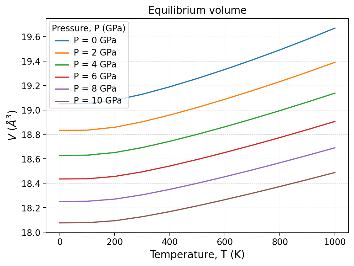
Equilibrium volume as a function of temperature for each pressure. The positive slope is thermal expansion; the downward displacement of the curves is pressure-induced compression. The curvature shows that expansion is not constant over the full temperature range.
Pressure sections at fixed temperature
When at least two pressure coordinates are stored, the complementary exact-grid view places pressure on the independent axis and selects stored temperatures:
quantas qha plot mgo_qha.hdf5 \
    --property VT \
    --property KT \
    --axis pressure \
    --temperature 300 \
    --temperature 1000 \
    --output qha_pressure_sections \
    --preset publication
These curves report \(V(P)\) and \(K_T(P)\) at fixed temperature. The temperature values must occur in the HDF5 grid exactly; no hidden interpolation or nearest-point selection is applied.
Heat capacities
quantas qha plot mgo_qha.hdf5 \
    --property heat_capacities \
    --energy-unit J/mol \
    --output qha_figures \
    --preset publication \
    --format png \
    --dpi 180
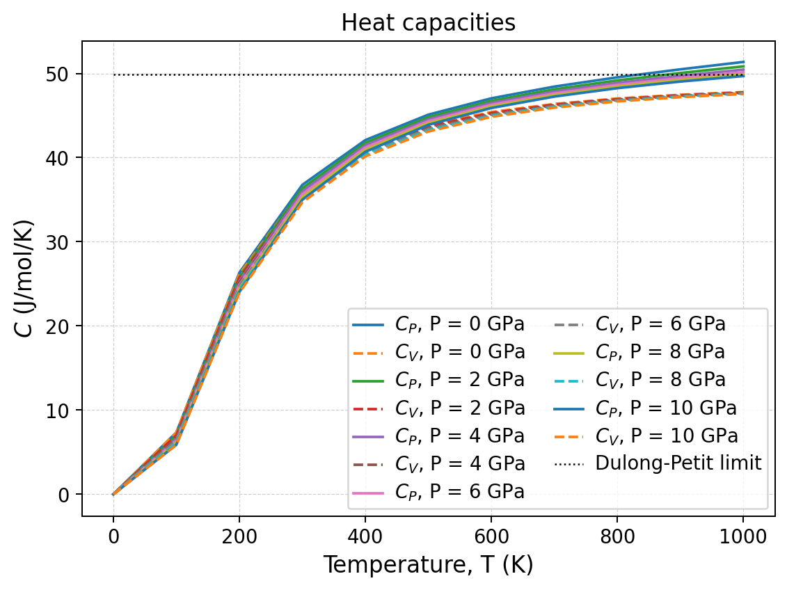
\(C_V\) is shown with dashed lines and \(C_P\) with solid lines. Their difference grows with temperature because thermal expansion couples heat input to mechanical work. The dotted horizontal line is the Dulong–Petit limit for two atoms per formula unit. The QHA \(C_P\) may exceed this harmonic classical limit because it includes the expansion term.
Pressure-temperature map of thermal expansion
quantas qha plot mgo_qha.hdf5 \
    --property alphaV \
    --2d \
    --cmap viridis \
    --levels 12 \
    --output qha_figures \
    --preset publication \
    --format png \
    --dpi 180
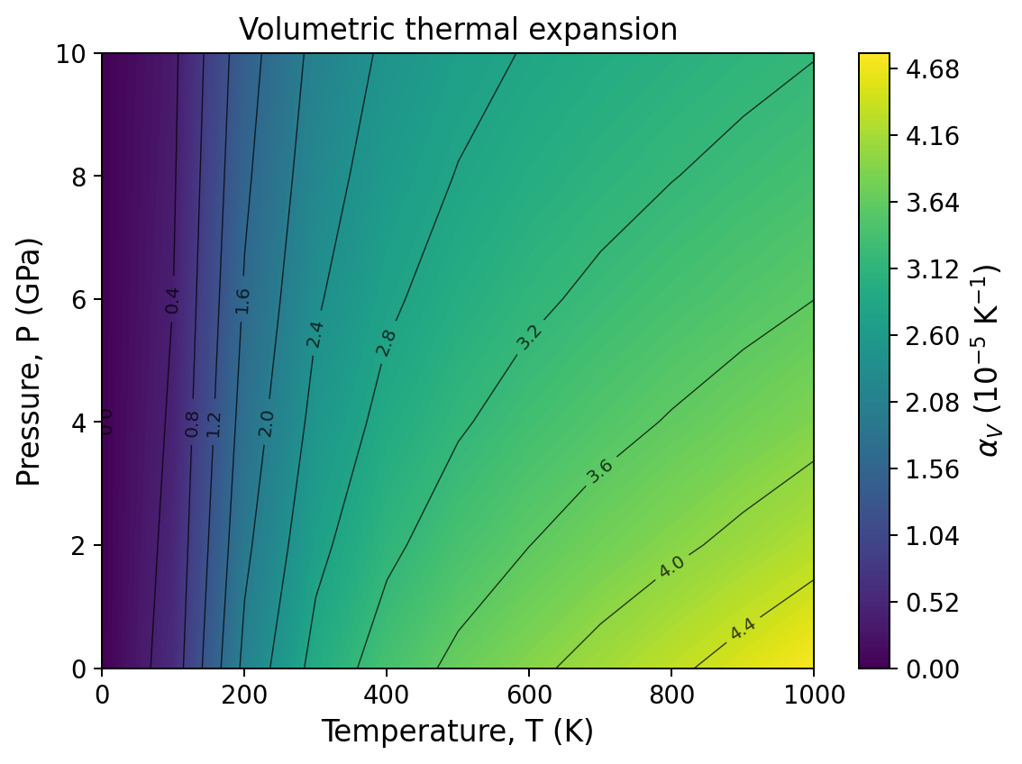
The contour map summarizes the coupled response. Expansion increases with temperature and decreases with pressure. The map must be interpreted only inside the calculated pressure-temperature domain and together with the input-volume coverage and workflow warnings.
Running the same calculation from Python
The public API reproduces the same scientific choices and result grids.
  1"""Reproduce the QHA MgO tutorial through the public Quantas API."""
  2
  3from __future__ import annotations
  4
  5import argparse
  6from pathlib import Path
  7
  8from quantas.api import qha, rendering
  9
 10
 11def main() -> None:
 12    """Inspect and run QHA, then write reports, HDF5, and selected figures."""
 13    parser = argparse.ArgumentParser()
 14    parser.add_argument("input", type=Path)
 15    parser.add_argument("--output-dir", type=Path, default=Path("qha_tutorial"))
 16    args = parser.parse_args()
 17
 18    args.output_dir.mkdir(parents=True, exist_ok=True)
 19
 20    options = qha.Options(
 21        temperature_min=0.0,
 22        temperature_max=1000.0,
 23        temperature_step=100.0,
 24        pressure_min=0.0,
 25        pressure_max=10.0,
 26        pressure_step=2.0,
 27        scheme="freq",
 28        minimization="poly",
 29        eos="BM3",
 30        energy_degree=3,
 31        free_energy_degree=3,
 32        frequency_degree=3,
 33        structural_degree=3,
 34        thermal_expansion_method="mixed_derivative",
 35        calculate_gruneisen=True,
 36        calculate_mode_gruneisen=True,
 37    )
 38
 39    preview = qha.inspect(
 40        args.input,
 41        options=options,
 42        include_polynomial=True,
 43        include_eos=True,
 44        polynomial_degree=3,
 45        eos="BM3",
 46    )
 47    print(
 48        "Static pressure coverage from BM3: "
 49        f"{preview.eos.pressure_min:.2f} to {preview.eos.pressure_max:.2f} "
 50        f"{preview.pressure_unit}"
 51    )
 52
 53    result = qha.run(args.input, options=options)
 54    payload = qha.get_result(result)
 55
 56    report = rendering.render_tables(qha.build_report(result))
 57    report_path = args.output_dir / "mgo_qha_api.log"
 58    report_path.write_text(report, encoding="utf-8")
 59
 60    hdf5_path = qha.write_result(
 61        result,
 62        args.output_dir / "mgo_qha_api.hdf5",
 63        report_text=report,
 64    )
 65
 66    volume_plots = qha.build_plots(
 67        result,
 68        properties=["VT"],
 69        options=qha.PlotOptions(),
 70    )
 71    rendering.render_plots(
 72        volume_plots,
 73        output_dir=args.output_dir,
 74        filename_prefix="mgo_qha_",
 75        preset="publication",
 76        dpi=180,
 77        close=True,
 78    )
 79
 80    heat_capacity_plots = qha.build_plots(
 81        result,
 82        properties=["heat_capacities"],
 83        options=qha.PlotOptions(energy_unit="J/mol"),
 84    )
 85    rendering.render_plots(
 86        heat_capacity_plots,
 87        output_dir=args.output_dir,
 88        filename_prefix="mgo_qha_",
 89        preset="publication",
 90        dpi=180,
 91        close=True,
 92    )
 93
 94    expansion_plots = qha.build_plots(
 95        result,
 96        properties=["alphaV"],
 97        options=qha.PlotOptions(
 98            include_contours=True,
 99            cmap="viridis",
100            levels=12,
101        ),
102    )
103    rendering.render_plots(
104        expansion_plots,
105        output_dir=args.output_dir,
106        filename_prefix="mgo_qha_",
107        preset="publication",
108        dpi=180,
109        close=True,
110    )
111
112    workflow = payload.metadata["workflow"]
113    print(f"Grid shape: {payload.temperature.size} x {payload.pressure.size}")
114    print(f"Successful points: {workflow['successful_points']}")
115    print(f"Failed points: {workflow['failed_points']}")
116    print(f"Written: {hdf5_path}")
117    print(f"Written: {report_path}")
118
119
120if __name__ == "__main__":
121    main()
Run it with:
python examples/qha/tutorial_api.py \
    examples/qha/crystal-qha/mgo_b3lyp.yaml \
    --output-dir qha_tutorial
The script first calls quantas.api.qha.inspect(), then runs QHA through
quantas.api.qha.run(). It writes a report and HDF5 result, builds the
same selected neutral plot specifications, and renders them using the public
rendering bridge.
Expected terminal summary:
Static pressure coverage from BM3: -15.29 to 48.88 GPa
Grid shape: 11 x 6
Successful points: 66
Failed points: 0
Written: qha_tutorial/mgo_qha_api.hdf5
Written: qha_tutorial/mgo_qha_api.log
Inspecting the typed result in Python
The module-specific payload exposes NumPy arrays without converting display precision into stored precision:
from quantas.api import qha

result = qha.read_result("mgo_qha.hdf5")
data = qha.get_result(result)

print(data.temperature.shape)       # (11,)
print(data.pressure.shape)          # (6,)
print(data.equilibrium_volume.shape)  # (11, 6)
print(data.thermal_expansion.shape)   # (11, 6)
print(data.lattice_parameters.shape)  # (11, 6, 6)
The arrays retain native float64 values. Formatting in reports and figures
is applied only by the renderers.
Exercise: sensitivity to interpolation and minimization
A QHA result is not determined only by the input data. It also depends on how the volume dependence is represented. Two independent choices are especially important:
freqortdinterpolation;polynomial or equation-of-state minimization of the free-energy curve.
This exercise compares the four combinations at 300 K and 0 GPa while keeping the input, polynomial degrees, thermal-expansion method, and pressure- temperature state unchanged.
Running the four CLI calculations
Use distinct result names so that no calculation overwrites another:
quantas qha run examples/qha/crystal-qha/mgo_b3lyp.yaml \
    --scheme freq --minimization poly \
    --temperature 300 300 1 --pressure 0 0 1 \
    --energy-degree 3 --frequency-degree 3 \
    --thermal-expansion mixed_derivative \
    --output qha_freq_poly.hdf5 --report qha_freq_poly.log \
    --no-progress --force

quantas qha run examples/qha/crystal-qha/mgo_b3lyp.yaml \
    --scheme td --minimization poly --no-mode-gruneisen \
    --temperature 300 300 1 --pressure 0 0 1 \
    --energy-degree 3 --frequency-degree 3 \
    --thermal-expansion mixed_derivative \
    --output qha_td_poly.hdf5 --report qha_td_poly.log \
    --no-progress --force

quantas qha run examples/qha/crystal-qha/mgo_b3lyp.yaml \
    --scheme freq --minimization eos --eos BM3 \
    --temperature 300 300 1 --pressure 0 0 1 \
    --energy-degree 3 --frequency-degree 3 \
    --thermal-expansion mixed_derivative \
    --output qha_freq_bm3.hdf5 --report qha_freq_bm3.log \
    --no-progress --force

quantas qha run examples/qha/crystal-qha/mgo_b3lyp.yaml \
    --scheme td --minimization eos --eos BM3 --no-mode-gruneisen \
    --temperature 300 300 1 --pressure 0 0 1 \
    --energy-degree 3 --frequency-degree 3 \
    --thermal-expansion mixed_derivative \
    --output qha_td_bm3.hdf5 --report qha_td_bm3.log \
    --no-progress --force
The same comparison can be automated through the public API:
Download the method-comparison script
python examples/qha/compare_methods.py \
    examples/qha/crystal-qha/mgo_b3lyp.yaml \
    --output qha_method_comparison.csv
Complete the table
Read the values from the reports or from the CSV produced by the script. The reference row is filled; complete the other rows before reading the discussion below.
Scheme |
Minimization |
EOS |
V (ų) |
\(K_T\) (GPa) |
\(\alpha_V\) (10⁻⁵ K⁻¹) |
\(C_V\) (J mol⁻¹ K⁻¹) |
\(C_P\) (J mol⁻¹ K⁻¹) |
\(\gamma\) |
|---|---|---|---|---|---|---|---|---|
freq |
poly |
– |
19.128633 |
163.53085 |
2.933514 |
36.27882 |
36.76515 |
1.52324 |
td |
poly |
– |
||||||
freq |
eos |
BM3 |
||||||
td |
eos |
BM3 |
What should be compared?
First compare freq and td at fixed minimization. For this curated MgO
dataset the two interpolation schemes agree very closely at 300 K: the volume
is identical at the shown precision and the differences in the principal
thermodynamic quantities are below about 0.05%. This indicates that fitting
mode-resolved frequencies or fitting the derived harmonic functions produces
nearly the same local free-energy surface for this state.
Next compare polynomial and BM3 minimization at fixed interpolation. The
change is larger: relative to freq/poly, freq/eos changes the volume by
about 0.24%, lowers \(K_T\) by about 3.1%, and raises
\(\alpha_V\) by about 3.7%. Heat capacities change much less. The main
sensitivity therefore comes from the curvature and minimum of the fitted
free-energy-volume relation, rather than from the harmonic thermodynamic
interpolation itself.
These percentages are properties of this dataset, volume interval, fit degree, EOS family, and selected state. They are not universal accuracy rankings. Agreement between methods increases confidence only when all fits are well-conditioned and the equilibrium volume remains inside the sampled range.
Optional extension: EOS-family sensitivity
Repeat the EOS rows with BM2, BM4, PT3 and V3. Add one row per
model and compare the fitted volume, curvature, and warning record. The purpose
is not to select the model that is numerically closest to the polynomial result,
but to determine whether scientifically reasonable EOS choices give stable
conclusions over the sampled compression range.
Reproducibility checkpoints
For the distributed input and the options used above:
all 66 pressure-temperature points complete successfully;
the BM3 inspection fit gives \(V_0\approx18.889084\) ų and \(K_0\approx167.81087\) GPa;
at 0 GPa and 300 K, \(V\approx19.128633\) ų and \(\alpha_V\approx2.933514\times10^{-5}\) K⁻¹;
at 10 GPa and 300 K, \(V\approx18.126469\) ų and \(\alpha_V\approx2.110356\times10^{-5}\) K⁻¹;
no structural extrapolation is reported for the selected grid;
the stored result records
mixed_derivativeas the source of all 66 thermal-expansion values.
Scientific limits
The tutorial validates reproducibility of this workflow, not universal validity of QHA. Before applying the same options to another material, examine:
dynamical stability and non-positive frequencies;
mode continuity when using the frequency scheme;
static and vibrational volume coverage;
fit quality and local failures;
extrapolation warnings;
phase transitions or strong intrinsic anharmonicity outside QHA.