Elasticity analysis

This tutorial analyzes the second-order elastic tensor of calcite. It follows one complete calculation from the text input to the native HDF5 result, the plain-text report, tabular export, and selected two- and three-dimensional figures. The same scientific workflow is then repeated through the public Python API.

The scientific background for the quantities used here is presented in Elasticity; the operational organization of the module is summarized in Elasticity analysis: implementation and workflow.

Scientific questions

The tutorial asks the following questions.

• Is the supplied stiffness tensor mechanically stable?

• What isotropic bulk, shear, and Young moduli would be assigned to a randomly oriented polycrystalline aggregate?

• How strongly do the single-crystal properties depend on direction?

• Which directions are mechanically soft or stiff?

• How do a principal-plane section and a complete three-dimensional surface represent the same directional property?

Dataset

The curated input is a B3LYP stiffness tensor for calcite. It is distributed with Quantas at examples/elasticity/calcite.dat.

Download calcite.dat

The file contains a job title followed by the upper triangular part of the stiffness matrix in Voigt notation. Elastic constants are expressed in GPa. A density may appear after the matrix so that the same text convention can be reused by SEISMIC; the Elasticity workflow itself reads the stiffness tensor.

Calcite (B3LYP)
  162.859000    63.582000    60.233000     0.000000    20.670000     0.000000
               162.859000    60.233000     0.000000   -20.670000     0.000000
                              89.647000     0.000000     0.000000     0.000000
                                           36.640000     0.000000   -20.670000
                                                        36.640000     0.000000
                                                                     49.638000
2680.000

The triangular representation is expanded to a symmetric \(6\times6\) matrix. The signs and positions of \(C_{15}\) and \(C_{46}\) encode the selected Cartesian representation of the trigonal tensor; they must not be silently removed or made positive.

Running Elasticity from the command line

Calculate the tensor characterization, exact directional extrema, and principal-plane fields:

quantas elasticity run examples/elasticity/calcite.dat \
    --2d \
    --ntheta 181 \
    --output calcite_elasticity.hdf5 \
    --report calcite_elasticity.log \
    --verbosity standard \
    --no-progress \
    --force

The calculation produces two complementary files.

calcite_elasticity.hdf5

Native scientific result containing the normalized input, options, stiffness and compliance tensors, averages, stability result, extrema, and sampled principal-plane data.

calcite_elasticity.log

Deterministic text rendering intended for inspection, archiving, and publication records. It is not a replacement for the structured HDF5 result.

The --2d option requests directional curves on the xy, xz, and yz planes. The global extrema reported by the workflow are not inferred from those three plots: Quantas calculates the transverse extrema using the full directional formulation.

Reading the report

Input and crystal system

The report first records the options and identifies the symmetry compatible with the matrix:

Elasticity input
----------------

     Property    |              Value
  ---------------+--------------------------------
  Job name       | Calcite (B3LYP)
  Crystal system | trigonal_low
  Source         | examples/elasticity/calcite.dat

The inferred crystal system is a diagnostic of the matrix pattern. It does not replace a crystallographic analysis of the original structure, and it depends on the tensor being supplied in the intended frame.

Stiffness and compliance

The stiffness matrix \(C\) is reported in GPa. Its inverse, the compliance matrix \(S=C^{-1}\), is also available in the complete report and HDF5 payload. Directional Young modulus, compressibility, shear modulus, and Poisson ratio are calculated from the compliance tensor.

Voigt–Reuss–Hill averages

For calcite, the report contains:

Voigt-Reuss-Hill average properties
-----------------------------------

  Scheme | K / GPa | E / GPa  | G / GPa |    nu
  -------+---------+----------+---------+---------
  Voigt  | 87.0512 | 104.0720 | 40.0047 | 0.300746
  Reuss  | 79.1474 | 81.0336  | 30.4784 | 0.329361
  Hill   | 83.0993 | 92.6302  | 35.2416 | 0.314218

The Voigt and Reuss estimates are upper and lower aggregate bounds under their respective assumptions. Their separation is itself useful: the larger spread in shear modulus than in bulk modulus indicates that the aggregate shear response is more sensitive to crystallographic orientation. The Hill values are arithmetic means of the two bounds; they describe an isotropic aggregate, not the directional response of one calcite crystal.

Mechanical stability

All six stiffness eigenvalues are positive:

Mechanical stability
--------------------

  Eigenvalue | Value / GPa
  -----------+------------
  1          | 21.471377
  2          | 25.117559
  3          | 48.800336
  4          | 64.806623
  5          | 110.799441
  6          | 267.287664

The tensor is therefore positive definite at the represented state. The smallest eigenvalue identifies the softest generalized elastic distortion, but it should not be interpreted as a particular Cartesian elastic constant.

Directional extrema

Selected results are:

Property	Minimum	Maximum	Maximum/minimum
Young modulus / GPa	57.6032	154.0608	2.6745
Linear compressibility / TPa⁻¹	2.2550	8.1246	3.6029
Shear modulus / GPa	21.4714	64.8069	3.0183
Poisson ratio	0.01139	0.76532	67.2133

The minimum Young modulus occurs along the input-frame \(z\) axis, whereas the stiffest direction is oblique to that axis. The compressibility is largest along \(z\), consistent with the comparatively soft longitudinal response normal to the calcite basal plane.

The very large maximum/minimum ratio reported for Poisson ratio must be read with care. Poisson ratio depends on both a loading direction and a transverse measurement direction. A small positive minimum makes a ratio-based anisotropy numerically large; the minimum and maximum values and their two associated directions are more informative than the ratio alone.

Exporting principal-plane data

The persisted 2D fields can be exported without repeating the calculation:

quantas elasticity export calcite_elasticity.hdf5 \
    --output calcite_elasticity_2d.dat

The file contains one block for each principal plane. Every row records the angular direction and the available branches of compressibility, shear modulus, Poisson ratio, and Young modulus. A shortened xy excerpt is:

# Plane: xy
# theta_deg phi_deg ... shear_modulus_1 shear_modulus_2 young_modulus
9.000000e+01 0.000000e+00 ... 2.803279e+01 3.797728e+01 9.980837e+01
9.000000e+01 2.000000e+00 ... 2.783666e+01 3.834327e+01 9.980837e+01

The two shear values correspond to the minimum and maximum transverse response for the selected propagation/loading direction. Young modulus has only one value for each direction.

Selected plots

Two-dimensional Young modulus

Render the three principal-plane sections from the stored result:

quantas elasticity plot calcite_elasticity.hdf5 \
    --2d \
    --property young \
    --preset publication \
    --dpi 180 \
    --output calcite_young

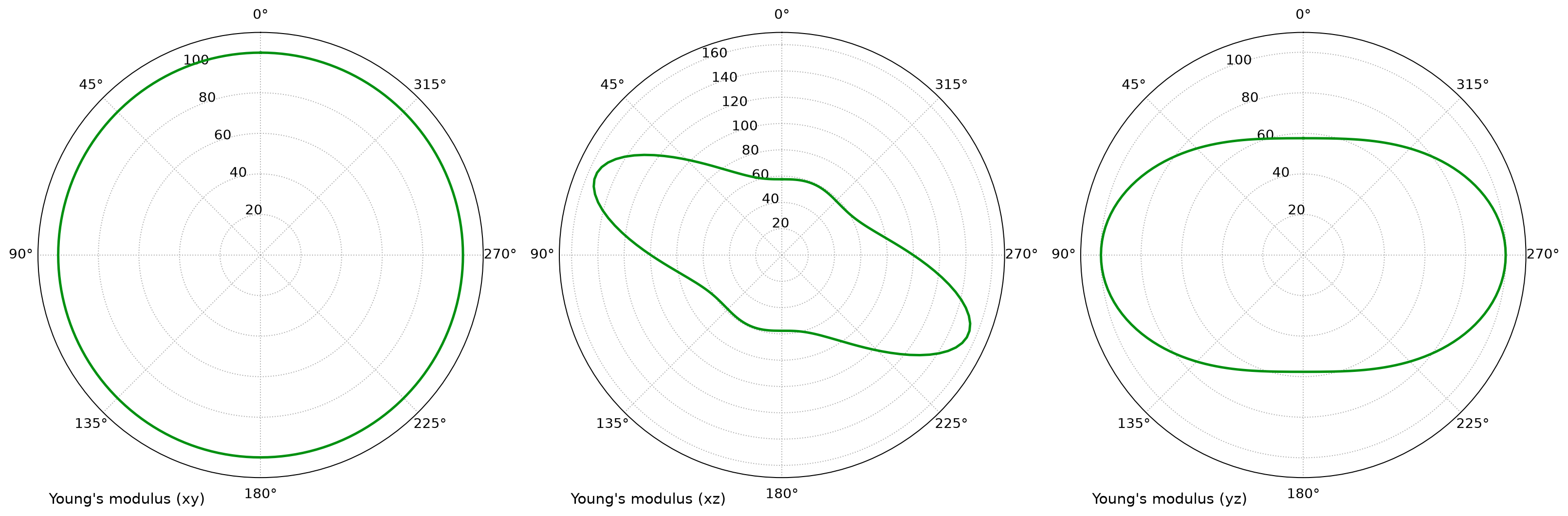
Young modulus of calcite on the xy, xz, and yz planes. The nearly circular basal-plane section reflects the threefold symmetry, while sections containing \(z\) reveal the much larger contrast between soft and stiff directions.

A 2D plot is an interpretable section, not a complete representation of the three-dimensional directional field. An extremum that lies outside the three selected planes need not be visible in these curves.

Three-dimensional physical surface

The complete Young-modulus surface can be rebuilt transiently from the stored tensor:

quantas elasticity plot calcite_elasticity.hdf5 \
    --3d \
    --property young \
    --geometry physical \
    --mesh \
    --mesh-color black \
    --mesh-linewidth 0.35 \
    --ntheta 61 \
    --nphi 121 \
    --preset publication \
    --dpi 180 \
    --output calcite_young_3d

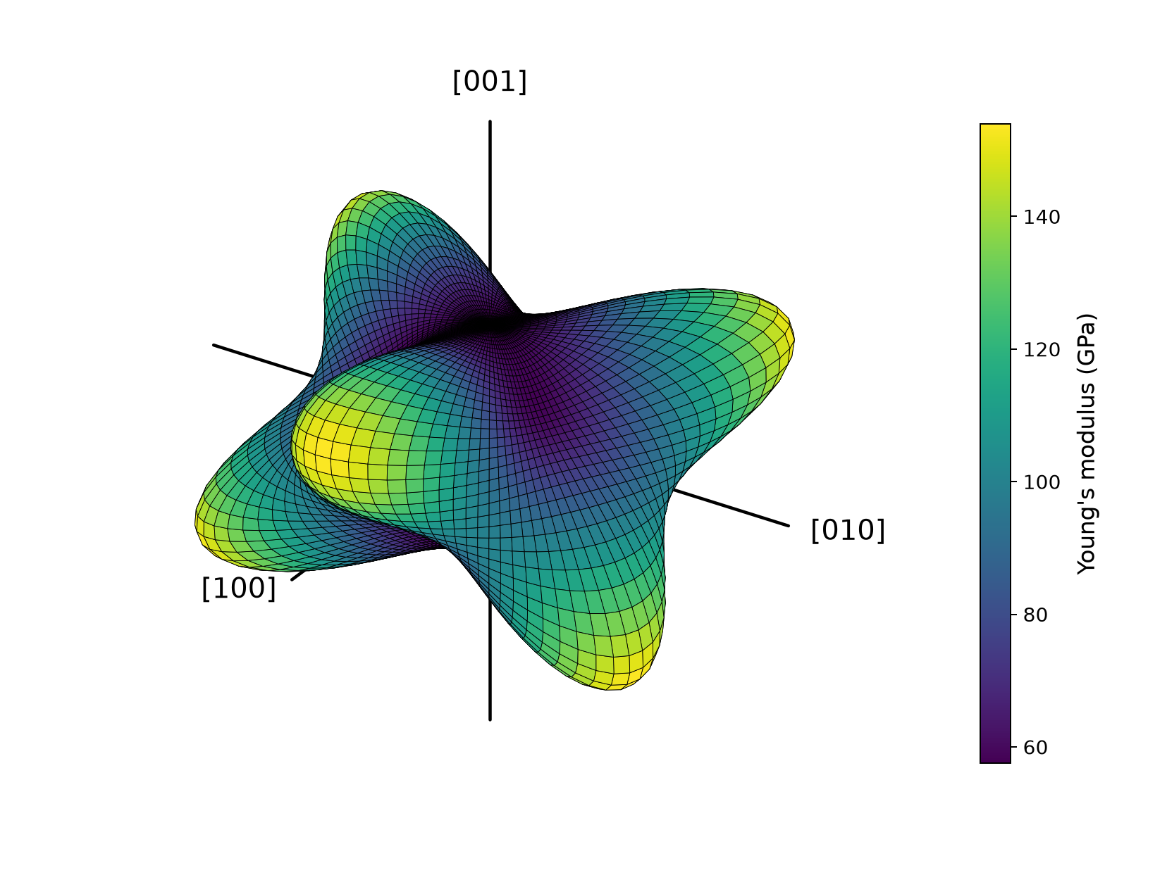
Physical Young-modulus surface. The radial distance and color both encode \(E(\mathbf n)\). Lobes identify stiff orientations; indentations identify soft orientations. Mesh lines show the angular sampling and are graphical aids rather than crystallographic planes.

With --geometry unit-sphere, the radius is fixed and only color carries the property value. That representation is often preferable when several properties must be compared on identical geometry.

Running the same workflow from Python

The complete script is distributed with the examples:

Download the Elasticity API script

"""Reproduce the Calcite Elasticity tutorial through the public Quantas API."""

from __future__ import annotations

import argparse
from pathlib import Path

from quantas.api import elasticity, rendering


def main() -> None:
    """Run the calculation, persist results, and render selected figures."""
    parser = argparse.ArgumentParser()
    parser.add_argument("input", type=Path)
    parser.add_argument(
        "--output-dir",
        type=Path,
        default=Path("elasticity_tutorial"),
    )
    args = parser.parse_args()

    args.output_dir.mkdir(parents=True, exist_ok=True)

    options = elasticity.Options(calculate_2d=True, ntheta=181)
    result = elasticity.run(args.input, options=options)
    payload = elasticity.get_result(result)

    report = rendering.render_tables(elasticity.build_report(result))
    report_path = args.output_dir / "calcite_elasticity_api.log"
    report_path.write_text(report, encoding="utf-8", newline="\n")
    hdf5_path = elasticity.write_result(
        result,
        args.output_dir / "calcite_elasticity_api.hdf5",
        report_text=report,
    )

    plots_2d = elasticity.build_2d_plots(
        result,
        properties=("young", "compressibility"),
    )
    rendering.render_plots(
        plots_2d,
        output_dir=args.output_dir,
        filename_prefix="calcite_",
        preset="publication",
        dpi=180,
        close=True,
    )

    plots_3d = elasticity.build_3d_plots(
        result,
        elasticity.SurfaceOptions(
            ntheta=61,
            nphi=121,
            properties=("young",),
        ),
        properties=("young",),
        geometry="physical",
        color_mode="property",
        show_mesh=True,
        mesh_color="black",
        mesh_line_width=0.35,
    )
    rendering.render_plots(
        plots_3d,
        output_dir=args.output_dir,
        filename_prefix="calcite_",
        preset="publication",
        dpi=180,
        close=True,
        axis_label_mode="crystal",
    )

    hill = payload.averages.hill
    young = payload.variations["young_modulus"]
    print(f"Crystal system: {payload.crystal_system}")
    print(f"Mechanically stable: {payload.stability.is_stable}")
    print(f"Hill bulk modulus / GPa: {hill.bulk_modulus:.6f}")
    print(f"Hill shear modulus / GPa: {hill.shear_modulus:.6f}")
    print(f"Young minimum / GPa: {young.minimum:.6f}")
    print(f"Young maximum / GPa: {young.maximum:.6f}")
    print(f"Written: {hdf5_path}")
    print(f"Written: {report_path}")


if __name__ == "__main__":
    main()

Run it from the repository root:

python examples/elasticity/tutorial_api.py \
    examples/elasticity/calcite.dat \
    --output-dir elasticity_tutorial

The script uses only the supported namespaces:

from quantas.api import elasticity, rendering

It performs the same sequence as the CLI:

1. read and normalize the text input;

2. construct quantas.api.elasticity.Options;

3. calculate the tensor properties;

4. obtain the typed result payload;

5. build and render the report;

6. write the native HDF5 result;

7. construct neutral 2D and 3D plot specifications;

8. render the figures with the public rendering entry point.

The final checkpoint output is:

Crystal system: trigonal_low
Mechanically stable: True
Hill bulk modulus / GPa: 83.099307
Hill shear modulus / GPa: 35.241563
Young minimum / GPa: 57.603207
Young maximum / GPa: 154.060777

Inspecting structured results

The HDF5 envelope can be reopened and converted to the typed payload:

from quantas.api import elasticity

result = elasticity.read_result("calcite_elasticity.hdf5")
payload = elasticity.get_result(result)

print(payload.crystal_system)
print(payload.stability.is_stable)
print(payload.averages.hill.bulk_modulus)
print(payload.variations["young_modulus"].minimum_axis)
print(payload.variations["young_modulus"].maximum_axis)

The raw numerical arrays remain available at full float64 precision. The number of displayed digits in a report or figure does not change the stored values.

CLI/API equivalence

The two frontends can be compared directly:

import numpy as np
from quantas.api import elasticity

cli = elasticity.get_result(
    elasticity.read_result("calcite_elasticity.hdf5")
)
api = elasticity.get_result(
    elasticity.read_result(
        "elasticity_tutorial/calcite_elasticity_api.hdf5"
    )
)

np.testing.assert_allclose(cli.stiffness, api.stiffness)
np.testing.assert_allclose(cli.compliance, api.compliance)
assert cli.averages == api.averages
assert cli.stability.is_stable == api.stability.is_stable

Reproducibility checkpoints

Using the distributed input without rotation, the following values should be reproduced to the displayed precision:

Quantity	Expected value
Crystal system	trigonal_low
Stable tensor	True
Hill \(K\) / GPa	83.099307
Hill \(G\) / GPa	35.241563
Minimum \(E\) / GPa	57.603207
Maximum \(E\) / GPa	154.060777
\(E_{\max}/E_{\min}\)	2.674517

Changing the angular resolution changes sampled curves and surfaces, but it must not change the stiffness matrix, compliance matrix, VRH averages, or exact directional-extrema calculation.

Further exploration

Useful extensions are:

• plot linear compressibility and identify the most compressible axis;

• plot minimum and maximum shear-modulus branches;

• inspect the two transverse directions associated with Poisson-ratio extrema;

• repeat the calculation after an explicit tensor rotation and verify that scalar extrema and VRH averages are invariant while their Cartesian directions rotate;

• compare physical and unit-sphere geometry for the same property.