Seismic wave analysis tutorial

Last updated

Jul 25, 2024

Author

Gianfranco Ulian

Preliminary operations

Download the hydroxylapatite input file, which contains the second-order elastic moduli tensor of hydroxylapatite in Voigt’s notation (values in GPa) and the density of the mineral, expressed in \(kg\ m^{-3}\). 1

Put this file in a folder of your choice and enter in this folder via the command prompt (or console under Linux/Mac OSX).

Analysis of the acoustic wave velocities by solving the Christoffel’s equation

This analysis is conducted in an automated mode by Quantas, so it is sufficient to type:

> quantas seismic hydroxylapatite.dat

to perform it.

Quantas reports the initial settings used in this analysis:

________                       __
\_____  \  __ _______    _____/  |______    ______
 /  / \  \|  |  \__  \  /    \   __\__  \  /  ___/
/   \_/.  \  |  // __ \|   |  \  |  / __ \_\___ \
\_____\ \_/____/(____  /___|  /__| (____  /____  >
       \__>          \/     \/          \/     \/
                                            v0.9.1
Authors: Gianfranco Ulian
Copyright 2020, University of Bologna


Calculator: wave velocities from Christoffel's equation

Measurement units
-------------------------------------
 - pressure:    GPa

Number of angular points
-------------------------------------
 - ntheta:      180
 - nphi:        720

Measurement units
-------------------------------------
 - pressure:    GPa

Plotting
-------------------------------------
 - requested:   True
 - dpi:         80
 - 3D plots:    True
 - 2D plots:    True
 - projection:  Lambert equal area

Warning

At the moment, only elastic constants expressed in GPa are supported. If you want to follow this tutorial with elastic constants for a system of your choice, and their value are not in GPa, please, convert them in this units before creating the input file and starting the analysis.

Then, the input file is read and relevant properties are printed on screen (and in the output file hydroxylapatite_SEISMIC.txt):

Reading input file: hydroxylapatite.dat
Analysis of the sound velocities in Hydroxylapatite

Stiffness matrix (values in GPa)
    187.2080       65.1930       84.7030        0.0000        0.0000        0.0000
     65.1930      187.2080       84.7030        0.0000        0.0000        0.0000
     84.7030       84.7030      222.6580        0.0000        0.0000        0.0000
      0.0000        0.0000        0.0000       39.6870        0.0000        0.0000
      0.0000        0.0000        0.0000        0.0000       39.6870        0.0000
      0.0000        0.0000        0.0000        0.0000        0.0000       61.0070

Compliance tensor (values in TPa^-1)
   6.758054    -1.437660    -2.023971     0.000000     0.000000     0.000000
  -1.437660     6.758054    -2.023971     0.000000     0.000000     0.000000
  -2.023971    -2.023971     6.031101     0.000000     0.000000     0.000000
   0.000000     0.000000     0.000000    25.197168     0.000000     0.000000
   0.000000     0.000000     0.000000     0.000000    25.197168     0.000000
   0.000000     0.000000     0.000000     0.000000     0.000000    16.391562

Then, the Quantas calculated the phase velocities, group velocities, power flow angle and the enhancement factor of the mineral along on different directions.

Start calculation of velocities by solving Christoffel's equation
  [##################################################]  100%

After this operation ended, both 3D (spherical) and 2D (polar) plots of the calculated properties are made.

Calculated data exported to hydroxylapatite_SEISMIC.hdf5
- making 3D plots of phase velocity
- making 2D plots of phase velocity
   *  Slow Secondary: anisotropy =  16.6 %
   *  Fast Secondary: anisotropy =  21.4 %
   *         Primary: anisotropy =  10.4 %
- making 3D plots of relative phase velocity
- making 2D plots of relative phase velocity
- making 3D plots of group velocity
- making 2D plots of group velocity
   *  Slow Secondary: anisotropy =  21.3 %
   *  Fast Secondary: anisotropy =  21.4 %
   *         Primary: anisotropy =  10.4 %
- making 3D plots of relative group velocity
- making 2D plots of relative group velocity
- making 3D plots of powerflow angle
- making 2D plots of powerflow angle
- making 3D plots of enhancement factor
- making 2D plots of enhancement factor
- making 2D plots of different ratios:
   * S-wave anisotropy = 200*(v_s1-v_s2)/(v_s1+v_s2)
   * v_P/v_s1
   * v_P/v_s2
- making 2D plots of polarization

The produced polar plots should be like the following ones:

Upper hemisphere equal area projection of the slow secondary, fast secondary and primary phase velocities.

Upper hemisphere equal area projection of the slow secondary, fast secondary and primary group velocities.

Upper hemisphere equal area projection of the slow secondary, fast secondary and primary power flow angle.

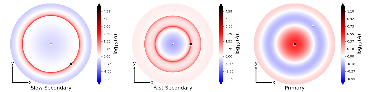
Upper hemisphere equal area projection of the slow secondary, fast secondary and primary enhancement factor.

Upper hemisphere equal area projection of the slow secondary, fast secondary and primary polarization of the phase velocities.

Note

The calculated data reported in the hydroxylapatite_SEISMIC.hdf5 contains the values used to generate the 2D and 3D plots of the elastic properties of the crystalline material. They can be extracted to generate plots according to the user’s preferences via:

quantas export seismic hydroxylapatite_SEISMIC.hdf5

References

1

Ulian, G., Valdre, G., 2018. Second-order elastic constants of hexagonal hydroxylapatite (P63) from ab initio quantum mechanics: comparison between DFT functionals and basis sets. Int. J. Quantum Chem. 118, e25500