Analysis of the acoustic wave propagation in crystalline solids

Overview

Second-order elastic moduli are typically obtained from Brillouin scattering techniques, which analyse the propagation of the acoustic (seismic) waves inside a crystalline material. Conversely, it is possible to obtain information on how the sound waves travel inside a homogeneous crystal by solving the Christoffel’s equation. In the following, a brief description of the theory and capabilities of Quantas within this framework is provided.

Last update

Jul 25, 2024

Author

Gianfranco Ulian

The basic property used to calculate the acoustic wave propagation in a homogeneous material (e.g., a perfect crystal) is the elastic tensor, which describes the relationship between stress \(\sigma\) and strain \(\epsilon\) according to the following formula:

(1)\[\sigma_{ij} = C_{ijkl} \epsilon_{kl}\]

where the \(C_{ijkl}\) terms are the component of the 3 \(\times\) 3 \(\times\) 3 \(\times\) 3 stiffness tensor 1. For the sake of clearness, all the sums here reported run over the three Cartesian coordinates x, y and z. Generally, Eq.(1) is written using the 6 \(\times\) 6 Voigt’s matrix notation of elastic tensor 1:

(2)\[\begin{split}\begin{equation} \begin{bmatrix} \sigma_{1} \\ \sigma_{2} \\ \sigma_{3} \\ \sigma_{4} \\ \sigma_{5} \\ \sigma_{6} \end{bmatrix} = \begin{bmatrix} C_{11} & C_{12} & C_{13} & C_{14} & C_{15} & C_{16} \\ C_{21} & C_{22} & C_{23} & C_{24} & C_{25} & C_{26} \\ C_{31} & C_{32} & C_{33} & C_{34} & C_{35} & C_{36} \\ C_{41} & C_{42} & C_{43} & C_{44} & C_{45} & C_{46} \\ C_{51} & C_{52} & C_{53} & C_{54} & C_{55} & C_{56} \\ C_{61} & C_{62} & C_{63} & C_{64} & C_{65} & C_{66} \end{bmatrix} \begin{bmatrix} \epsilon_{1} \\ \epsilon_{2} \\ \epsilon_{3} \\ 2\epsilon_{4} \\ 2\epsilon_{5} \\ 2\epsilon_{6} \end{bmatrix} \end{equation}\end{split}\]

with the subscripts being mapped as 1 = \(xx\), 2 = \(yy\), 3 = \(zz\), 4 = \(yz\), 5 = \(xz\), 6 = \(xy\), and the double counting is accounted by the factor 2 in the strain tensor.

To access information on the elastic (acoustic) waves that travel through the material, it is necessary to solve Christoffel’s equation 2. Let’s define \(\textbf{q}\) a monochromatic wave vector with angular frequency \(\omega\) and polarization \(\boldsymbol{\hat{\mathbf{p}}}\) that travels inside a crystalline material with density \(\rho\). The Christoffel equation is an eigenvalue problem defined as:

(3)\[\sum_{ij} \bigg[ M_{ij} - \rho \omega^2 \delta_{ij} \bigg] s_j = 0\]

where \(M_{ij}\) are the terms of the Christoffel’matrix \(\textbf{M}\) that are written as

(4)\[M_{ij} = \sum_{kl} q_k C_{iklj} q_j\]

Eq.(3) can be solved for any given \(\textbf{q}\). From now on, the notation suggested by Jaeken and Cottenier will be used 3, which introduces the reduced stiffness tensor \(\textbf{C}' = \textbf{C} / \rho\) and the reduced Christoffel matrix \(\textbf{M}' = \textbf{M} / \rho\). For convenience, the prime on these two tensor quantities will be dropped. In addition, Eq.(3) and Eq.(4) show \(\omega (\textbf{q})\) is a linear function of \(\textbf{q}\) in a single direction, which means the sound velocities are independent of the wavelength \(\textbf{q}\) but its direction. Hence, \(\textbf{q}\) will be considered from now on a dimensionless unit vector that describes only the travel direction of the monochromatic plane wave. These considerations lead to the following formula:

(5)\[\sum_{ij} \bigg[ M_{ij} - \nu_p^2 \delta_{ij} \bigg] s_j = 0\]

with \(\nu_p\) the velocity of the monochromatic plane wave that travels in the direction given by \(\boldsymbol{\hat{\mathbf{q}}}\). The subscript \(p\) denotes this quantity as the phase velocity. The non-trivial solutions of Eq.(5) are three eigenvalues, i.e. three velocities subdivided into one primary (P-mode) and two secondary (S-mode), which are related to the (pseudo-) longitudinal and (pseudo-)transversal polarizations, respectively. As a convention, the two secondary velocities are one fast S-mode and a slow S-mode, so that in general \(\nu_{p,P} > \nu_{p,S_{fast}} > \nu_{p,S_{slow}}\), and the difference \(\nu_{p,S_{fast}} - \nu_{p,S_{slow}}\) is called shear-wave splitting. The three eigenvector solutions of the Christoffel equation are associated with the polarization directions.

The above formulas consider the sound as a monochromatic plane wave, an ideal situation. Indeed, real sound could be considered as a wave packet whose wavelength and travelling direction show a certain amount of spreading. Thus, the sound (acoustic energy) travels through a homogeneous medium as a wave packet given by the superposition of several phase waves, whose velocity is described by the following formula:

(6)\[\textbf{v}_g = \vec{\nabla} \nu_p\]

where \(\textbf{v}_g\) is the so-called group velocity, whose direction is the travel direction of (acoustic) energy if the medium does not dissipate energy. The gradient (in reciprocal space) is given by the derivative of the components of the dimensionless vector \(\boldsymbol{\hat{\mathbf{q}}}\). It is worth noting that \(\textbf{v}_g\) is a vector that typically does not line in the direction of \(\boldsymbol{\hat{\mathbf{q}}}\), and the power flow angle \(\psi\) describes the angular difference between the directions of the group and phase velocity according to:

(7)\[\nu_p = \nu_g \cos ( \psi )\]

If we introduce the normalized directions of the phase velocity, \(\boldsymbol{\hat{\mathbf{n}}}_p\), and of the group velocity, \(\boldsymbol{\hat{\mathbf{n}}}_g\), we can re-write Eq.(7) as:

(8)\[\cos ( \psi ) = \boldsymbol{\hat{\mathbf{n}}}_p \cdot \boldsymbol{\hat{\mathbf{n}}}_g\]

Since the energy travelling direction typically is not the same of the phase velocity, the power flow concentration changes depending on the direction, with the enhancement factor \(A\) providing the quantification of this effect according to:

(9)\[A = \frac {\Delta \Omega_p} {\Delta \Omega_g}\]

In Eq.(9), \(\Omega_p\) and \(\Omega_g\) are the solid angles subtended by beams of phase \(\boldsymbol{\hat{\mathbf{n}}}_p\) and group \(\boldsymbol{\hat{\mathbf{n}}}_g\) wave vectors, respectively.

The most simple way to determine the enhancement factor is to consider its infinitesimal value, which is easily described in spherical coordinates, as suggested by Jaeken and Cottenier 3. With this approach, the solid angle is equal to the area of a quadrangle described on the unit sphere by the partial derivatives of the phase vector \(\boldsymbol{\hat{\mathbf{n}}}_p\) or group vector \(\boldsymbol{\hat{\mathbf{n}}}_p\) to \(\theta\) and \(\phi\). This translates into

(10)\[d \Omega_p = \sin ( \theta ) d \theta d \phi\]

and

(11)\[d \Omega_g = \left\lVert \frac {\partial \boldsymbol{\hat{\mathbf{n}}}_g} {\partial \theta} \times \frac {\partial \boldsymbol{\hat{\mathbf{n}}}_g} {\partial \phi} \right\rVert \sin ( \theta ) d \theta d \phi\]

Thus, the enhancement factor is given by

(12)\[A = \left\lVert \frac {\partial \boldsymbol{\hat{\mathbf{n}}}_g} {\partial \theta} \times \frac {\partial \boldsymbol{\hat{\mathbf{n}}}_g} {\partial \phi} \right\rVert^{-1},\]

which can be also expressed as

(13)\[\begin{split}\big( \hat{\theta} \cdot \vec{\nabla} \boldsymbol{\hat{\mathbf{n}}}_g \big) \times \big( \hat{\phi} \cdot \vec{\nabla} \boldsymbol{\hat{\mathbf{n}}}_g \big) = & \big| \vec{\nabla} \boldsymbol{\hat{\mathbf{n}}}_g \big| \big( \vec{\nabla} \boldsymbol{\hat{\mathbf{n}}}_g \big)^{-T} \cdot \big( \hat{\theta} \times \hat{\phi} \big) \\ = & \big| \vec{\nabla} \boldsymbol{\hat{\mathbf{n}}}_g \big| \big( \vec{\nabla} \boldsymbol{\hat{\mathbf{n}}}_g \big)^{-T} \cdot \boldsymbol{\hat{\mathbf{q}}} \\ = & \mathbf{Cof} (\vec{\nabla} \boldsymbol{\hat{\mathbf{n}}}_g) \cdot \boldsymbol{\hat{\mathbf{q}}}\end{split}\]

where Cof() indicates the matrix of cofactors, and

(14)\[\begin{split}\hat{\theta} = \frac {\partial \hat{\mathbf{q}}} {\partial \theta}, \\ \hat{\phi} = \frac {\partial \hat{\mathbf{q}}} {\partial \phi}. \\\end{split}\]

By substituting Eq.(13) into Eq.(14), the enhancement factor is given by the following expression

(15)\[A = \left\lVert \mathbf{Cof} \big( \vec{\nabla} \boldsymbol{\hat{\mathbf{n}}}_g \big) \right\rVert^{-1},\]

which is not dependent on the spherical coordinates and can be evaluated from the derivatives of the Christoffel’s matrix eigenvalues.

Workflow of elastic constant analysis

The following picture shows a schematic workflow of the analysis of the second-order elastic moduli to obtain the seismic wave velocities.

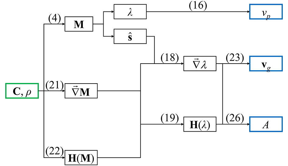
The green box reports the input data (tensor of the elastic moduli in Voigt’s notation and crystal density), whereas the blue ones are the output of the calculation. The numbers in parentheses are references to the equations shown along the text.

As previously suggested 3, the implemented computational approach uses the eigenvalues of the Christoffel’s matrix, \(\lambda\), as the key quantity to obtain all the measurable properties (phase velocity \(\nu_p\), group velocity \(\nu_g\) and enhancement factor A). Hence, the phase velocity is defined as

(16)\[\nu_p = \sqrt{ \lambda }\]

that can be substituted in Eq.(6) to give

(17)\[\textbf{v}_g = \vec{\nabla} \nu_p = \vec{\nabla} \sqrt{ \lambda } = \frac {\vec{\nabla} \lambda} {2 \sqrt{ \lambda }}.\]

Except for the phase velocities, all the other quantities are obtained from the first and second derivatives of the matrix \(\lambda\). The gradient of the generic eigenvalue \(\lambda_i\) can be expressed as

(18)\[\frac{\partial \lambda_i}{\partial q_k} = \boldsymbol{\hat{\mathbf{s}}}_i \cdot \frac {\partial \mathbf{M}}{\partial q_k} \cdot \boldsymbol{\hat{\mathbf{s}}}_i\]

with \(\boldsymbol{\hat{\mathbf{s}}}_i\) the normalized eigenvector related to \(\lambda_i\). The Hessian matrix \(\mathbf{H}(\lambda)\) is given by the second-order derivatives of the Christoffel’s eigenvalues, according to the following expression

(19)\[\mathbf{H}(\lambda_i) = \frac{\partial^2 \lambda_i}{\partial q_k \partial q_m} = \boldsymbol{\hat{\mathbf{s}}}_i \cdot \frac{\partial^2 \mathbf{M}}{\partial q_k \partial q_m} \cdot \boldsymbol{\hat{\mathbf{s}}}_i + 2\boldsymbol{\hat{\mathbf{s}}}_i \cdot \frac{\partial \mathbf{M}}{\partial q_k} \cdot \big( \lambda_i \mathbf{I} - \mathbf{M} \big)^{+} \cdot \frac{\partial \mathbf{M}}{\partial q_m} \cdot \cdot \boldsymbol{\hat{\mathbf{s}}}_i\]

which is obtained from the derivative of the gradient of the eigenvectors given by 4

(20)\[\frac{\boldsymbol{\hat{\mathbf{s}}}_i}{\partial q_k} = \big( \lambda_i \mathbf{I} - \mathbf{M} \big)^{+} \cdot \frac{\partial \mathbf{M}}{\partial q_k} \cdot \cdot \boldsymbol{\hat{\mathbf{s}}}_i\]

In this framework, the derivative of the Christoffel’s matrix, \(\vec{\nabla} \mathbf{M}\) (third-order tensor), is simply

(21)\[\vec{\nabla} \mathbf{M} = \frac{\partial M_{ij}}{\partial q_k} = \sum_m \big( C_{ikmj} + C_{imkj} \big) q_m,\]

and its Hessian is

(22)\[\mathbf{H}(\mathbf{M}) = \frac {\partial^2 M_{ij}}{\partial q_k \partial q_m} = C_{ikmj} + C_{imkj}.\]

It is worth noting that (i) Eq.(21) depends on q, whereas Eq.(22) does not, and (ii) the group velocities can be straightforwardly obtained from the solution of Eq.(21), Eq.(18), and Eq.(17), which require just the eigenvalues and eigenvectors of \(\mathbf{M}\):

(23)\[\mathbf{v}_g^i = \frac { \boldsymbol{\hat{\mathbf{s}}}_i \cdot \vec{\nabla} \mathbf{M} \cdot \boldsymbol{\hat{\mathbf{s}}}_i} {2 \sqrt{\lambda_i}}.\]

The calculation of the enhancement factor considers the gradient of the vector field of the normalized group velocity with respect to \(\lambda\),

(24)\[\vec{\nabla} \boldsymbol{\hat{\mathbf{n}}}_g = \vec{\nabla} \frac {\mathbf{v}_g} { \lVert \mathbf{v}_g \rVert } = \vec{\nabla} \frac {\vec{\nabla} \nu_p} { \lVert \vec{\nabla} \nu_p \rVert } = \vec{\nabla} \frac {\vec{\nabla} \lambda} { \lVert \vec{\nabla} \lambda \rVert }.\]

Considering that the gradient of a differentiable and positive vector field v is given by

(25)\[\vec{\nabla} \frac {\mathbf{v}}{\lVert \mathbf{v} \rVert} = \frac {\vec{\nabla} \mathbf{v}}{\lVert \mathbf{v} \rVert} - \frac {\mathbf{v} \otimes \big( \vec{\nabla} \mathbf{v} \big) \cdot \mathbf{v}} {\lVert \mathbf{v} \rVert^3},\]

where \(\otimes\) is the Kronecker’s product, it follows that

(26)\[\vec{\nabla} \boldsymbol{\hat{\mathbf{n}}}_g = \frac{\mathbf{H}(\lambda)} {\lVert \vec{\nabla} \lambda \rVert} - \frac {\vec{\nabla} \lambda \otimes \mathbf{H}(\lambda) \times \vec{\nabla} \lambda} {\lVert \vec{\nabla} \lambda \rVert^3},\]

It is important to highlight that the outer product in Eq.(26) does not commute, hence is not equal to its transposed matrix, i.e., the matrix is not symmetric 3.

References

1(1,2)

Nye, J.F., 1957. Physical properties of crystals. Oxford University Press, Oxford.

2

Musgrave, M.F.P., 1970. Crystal Acoustics: Introduction to the Study of Elastic Waves and Vibrations in Crystals, Holden-Day, San Francisco, CA, USA.

3(1,2,3,4)

Jaeken J.W, Cottenier S., 2016. Solving the Christoffel equation: Phase and group velocities. Comput. Phys. Commun. 207, 445-451.

4

Petersen K.B., Pedersen M.S., 2012. The Matrix Cookbook. Version 15 November 2012. http://matrixcookbook.com