Second-Order Elastic Moduli Analysis tutorial
- Last updated
Jul 25, 2024
- Author
Gianfranco Ulian
Preliminary operations
Download the hydroxylapatite input file,
which contains the second-order elastic tensor of hydroxylapatite in Voigt
notation (\(6 \times 6\) matrix, values in GPa) and the density of the mineral,
expressed in \(kg\ m^{-3}\). 1
Put this file in a folder of your choice and enter in this folder via the command prompt (or console under Linux/Mac OSX).
Analysis of the second-order elastic constants
This analysis is conducted in an automated mode by Quantas, so it is sufficient to type:
> quantas soec hydroxylapatite.dat
to perform it.
Quantas reports the initial settings used in this analysis:
________                       __
\_____  \  __ _______    _____/  |______    ______
 /  / \  \|  |  \__  \  /    \   __\__  \  /  ___/
/   \_/.  \  |  // __ \|   |  \  |  / __ \_\___ \
\_____\ \_/____/(____  /___|  /__| (____  /____  >
       \__>          \/     \/          \/     \/
                                            v0.9.0
Authors: Gianfranco Ulian
Copyright 2020, University of Bologna


Calculator: Second-order elastic constants analysis

Measurement units
-------------------------------------
 - pressure:    GPa
Warning
At the moment, only elastic constants expressed in GPa are supported. If you want to follow this tutorial with elastic constants for a system of your choice, and their value are not in GPa, please, convert them in this units before creating the input file and starting the analysis.
Then, the input file is read and relevant properties are printed on screen (and in the output
file hydroxylapatite_SOEC.txt):
Reading input file: hydroxylapatite.dat

Elastic analysis of Hydroxylapatite

System is hexagonal
Density: 3178.0 kg m^-3

Stiffness matrix (values in GPa)
    187.2080       65.1930       84.7030        0.0000        0.0000        0.0000
     65.1930      187.2080       84.7030        0.0000        0.0000        0.0000
     84.7030       84.7030      222.6580        0.0000        0.0000        0.0000
      0.0000        0.0000        0.0000       39.6870        0.0000        0.0000
      0.0000        0.0000        0.0000        0.0000       39.6870        0.0000
      0.0000        0.0000        0.0000        0.0000        0.0000       61.0070

Compliance tensor (values in TPa^-1)
   6.758054    -1.437660    -2.023971     0.000000     0.000000     0.000000
  -1.437660     6.758054    -2.023971     0.000000     0.000000     0.000000
  -2.023971    -2.023971     6.031101     0.000000     0.000000     0.000000
   0.000000     0.000000     0.000000    25.197168     0.000000     0.000000
   0.000000     0.000000     0.000000     0.000000    25.197168     0.000000
   0.000000     0.000000     0.000000     0.000000     0.000000    16.391562
A symmetry analysis on the values of the SOECs matrix (correctly) revealed that the system is hexagonal, and the stiffness and compliance matrices are reported.
Polycrystalline (average) properties:
Average properties
          Bulk      Young's      Shear     Poisson's
        modulus     modulus     modulus      ratio
         (GPa)       (GPa)       (GPa)
Voigt  118.47467   136.63989    52.24120    0.30778
Reuss  116.60441   131.05436    49.91864    0.31268
Hill   117.53954   133.85036    51.07992    0.31021
and the eigenvalues of the stiffness matrix:
Eigenvalues of the stiffness matrix:
    lambda_1: 39.68700
    lambda_2: 39.68700
    lambda_3: 61.00700
    lambda_4: 116.82176
    lambda_5: 122.01500
    lambda_6: 358.23724
are calculated and reported. The eigenvalues are all positive, meaning that the system is mechanically stable.
Note
If any of the eigenvalues were negative, the analysis would have stopped, detecting the instability of the system.
Quantas then proceeds searching for the minimum and maximim values of:
Young’s modulus;
linear compressibility;
shear modulus;
Poisson’s ratio
seismic waves (if the density is present in input)
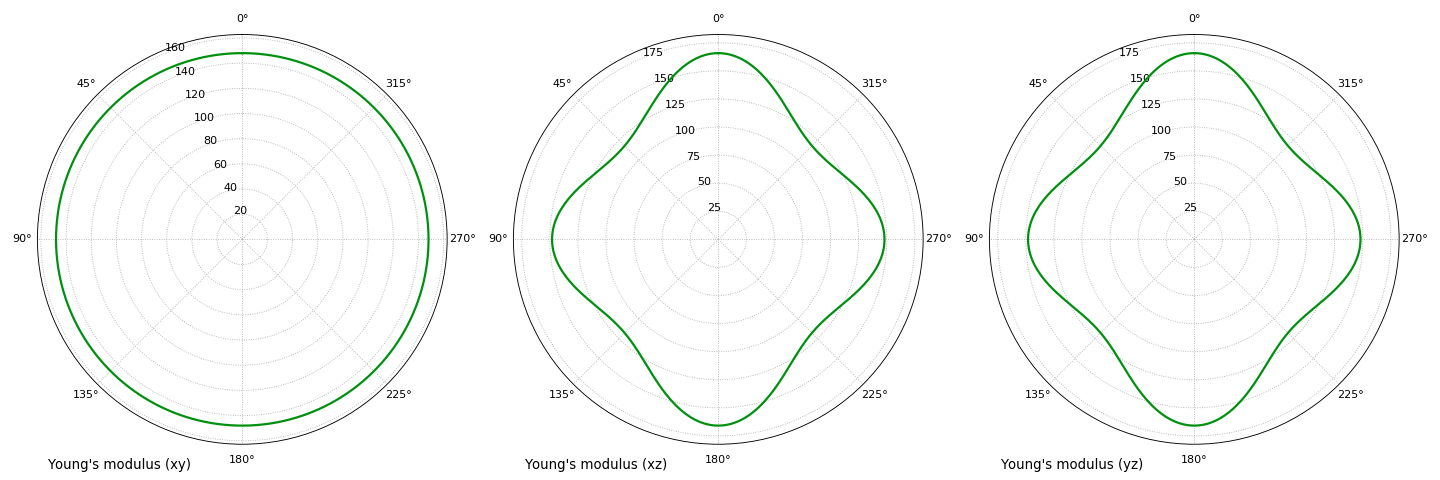
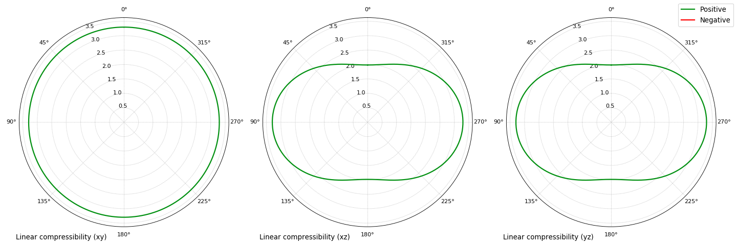
along crystal directions, assuming the system as a monocrystal. The results of this procedure are reported in tabular format for Young’s modulus and linear compressibility:
Variations of the elastic moduli:

    --------------------------------------------------------------------------------
               |         Young's modulus          |      Linear compressibility
    -----------|----------------------------------|---------------------------------
               |      E_min            E_max      |    beta_min         beta_max
    Values     |    117.6414         165.8072     |     1.9832           3.2964
    -----------|----------------------------------|---------------------------------
    Anisotropy |              1.4094              |              1.6622
    -----------|----------------------------------|---------------------------------
               |     0.5213           0.0000      |     0.0000           0.7071
    Axis       |     0.5213           0.0000      |     0.0000           0.7071
               |     0.6757           1.0000      |     1.0000           0.0000
    --------------------------------------------------------------------------------
Notes: E min/max values in GPa, beta min/max values in TPa^-1
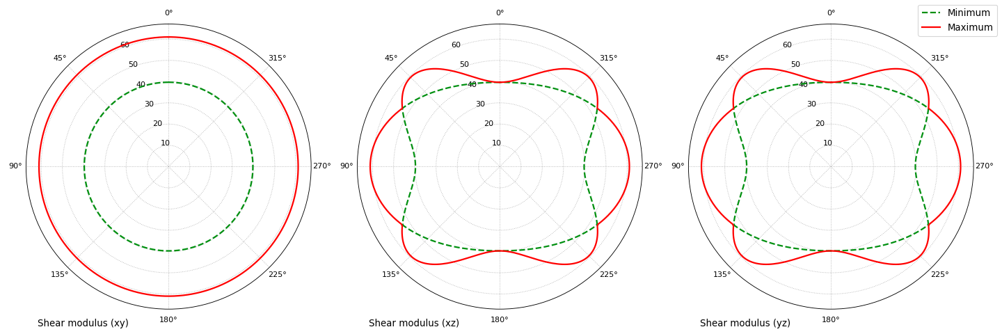
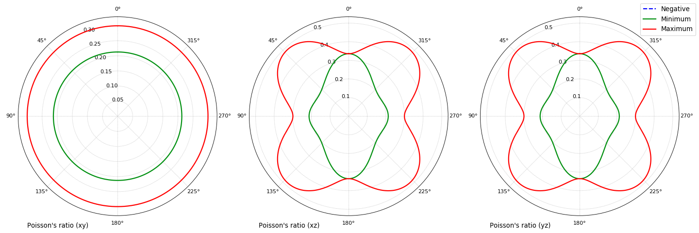
for shear modulus and Poisson’s ratio:
    --------------------------------------------------------------------------------
               |          Shear modulus           |         Poisson's ratio
    -----------|----------------------------------|---------------------------------
               |      G_min            G_max      |     nu_min           nu_max
    Values     |     39.6870          61.0075     |     0.1944           0.4857
    -----------|----------------------------------|---------------------------------
    Anisotropy |              1.5372              |              2.4987
    -----------|----------------------------------|---------------------------------
               |     0.5000           -0.6832     |     0.0000           0.7356
    1st Axis   |     0.8660           0.7302      |     -1.0000          -0.0002
               |     0.0000           0.0000      |     -0.0000          -0.6775
    -----------|----------------------------------|---------------------------------
               |     0.5000           -0.6832     |     0.0000           0.7356
    2nd Axis   |     0.8660           0.7302      |     -1.0000          -0.0002
               |     0.0000           0.0000      |     -0.0000          -0.6775
    --------------------------------------------------------------------------------
Notes: G min/max values in GPa
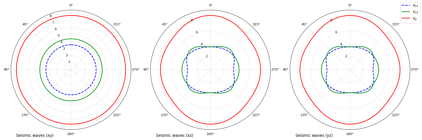
and for seismic wave velocities:
Variations of the seismic velocities:

    -------------------------------------------------------------------------------------
               |          V_s1          |          V_s2          |          V_p
    -----------|------------------------|------------------------|-----------------------
               |    min         max     |    min         max     |    min         max
    Values     |   3.5338      4.1768   |   3.5338      4.3814   |   7.5397      8.3703
    -----------|------------------------|------------------------|-----------------------
    Anisotropy |         1.1819         |         1.2398         |         1.1102
    -----------|------------------------|------------------------|-----------------------
               |   0.0000      0.8597   |  -0.0000      0.7071   |   0.5987      0.0000
    Axis       |  -0.0000     -0.0000   |  -0.0000      0.7071   |   0.5987      0.0000
               |  -1.0000      0.5109   |   1.0000      0.0000   |  -0.5320     -1.0000
    -------------------------------------------------------------------------------------
Notes: min/max values in km s^-1
Analysis of elastic properties on \((xy)\), \((xz)\) and \((yz)\) planes
By using the --polar option, the elastic properties are evaluated on the cited planes:
> quantas soec hydroxylapatite.dat --polar
The analysis proceeds calculating the bi-dimensional variations of the cited properties on the \((xy)\), \((xz)\) and \((yz)\) planes:
- Calculation of polar (2D) properties:
    * along (xy)
        a. Young's modulus
        b. Linear compressibility
        c. Shear modulus
        d. Poisson's ratio
        e. Wave velocities
    * along (xz)
        a. Young's modulus
        b. Linear compressibility
        c. Shear modulus
        d. Poisson's ratio
        e. Wave velocities
    * along (yz)
        a. Young's modulus
        b. Linear compressibility
        c. Shear modulus
        d. Poisson's ratio
        e. Wave velocities

 Calculation time:     62.7 sec
Some polar plots of the elastic properties can be produced in an automated mode if the command is launched as:
> quantas soec hydroxylapatite.dat --polar --plot
Note
To generate publication-ready picture, it is recommended to increase the dot-per-inch (DPI) of the output images by using, for example:
> quantas soec hydroxylapatite.dat --polar --plot --dpi 300
If plots are requested, the following lines will be printed:
Plotting results as requested:
 - figure hydroxylapatite_SOEC_E.png generated
 - figure hydroxylapatite_SOEC_LC.png generated
 - figure hydroxylapatite_SOEC_G.png generated
 - figure hydroxylapatite_SOEC_Nu.png generated
 - figure hydroxylapatite_SOEC_waves.png generated

Calculated data exported to hydroxylapatite_SOEC.hdf5
The produced polar plots should be like the following ones:
Note
The calculated data reported in the hydroxylapatite_SOEC.hdf5 contains the values used to
generate the 2D polar plots of the elastic properties of the crystalline material. They can
be extracted to generate plots according to the user’s preferences via:
quantas export soec hydroxylapatite_SOEC.hdf5
References
- 1
Ulian, G., Valdre, G., 2018. Second-order elastic constants of hexagonal hydroxylapatite (P63) from ab initio quantum mechanics: comparison between DFT functionals and basis sets. Int. J. Quantum Chem. 118, e25500